Chapter 20 Mapping and analysing pine densities at Arne
20.1 Introduction
This handout aims to step through most of the work for the assignment.
20.1.1 Loading libraries
The first step as always is to set up a chunk which loads the libraries. Some of the libraries send warning messages that are printed in the knitted document. To avoid them set some knit options by copying the line below into the very first chunk.
knitr::opts_chunk$set(echo = TRUE,message = FALSE,warning = FALSE)library(aqm)
library(giscourse)
library(raster)
library(ggplot2)
library(sf)
library(tmap)
library(mapview)
library(dplyr)
library(mgcv)20.2 Loading the data
The data we are going to use consists of numbers of pines counted in circular quadrats over three years of field work. The first survey took place in 2017. At that time pines were growing throughout the heathland. The students decided to sample them through a “random walk” transect design in order to cover as much of the area as possible. As we saw in the field, many of the pines have been removed from Coombe heath since then. So in 2018 and 2019 the survey concentrated on smaller areas that had not been pulled.
data("arne_pines")What do these data consist of?
We can answer the question by clicking on the object in the global Environment window. Or we can add the data to the knitted document itself using the dt function
dt(arne_pines)20.2.1 Points to notice
- Notice that the site is a factor with two levels. Heath and restoration. In other words all the quadrats in Coombe’s heath are labeled as coming from heath and those in the restoration site are labeled. The restoration site was only measured in the last survey, so this will be treated rather differently in the analysis.
- The pine_density variable has been calculated by dividing the number of pines by the area of the quadrat. Last year the students decided to use smaller quadrats, so the counts of pine numbers are not directly comparable until they have been standardised in this way. The pine density multipied by an area in square meters produces an estimate of the total number of pines.
- There are coordinates of the quadrats as longitude (lon) and lattitude (lat). This is the most universal way of storing spatial data. It is easy to convert these to national grid when we need to measure areas and distances.
20.2.2 Making a spatial object in R
The data as they stand are not yet in a GIS format. They are just a data frame that can be opened in Excel, or any other similar program. There is spatial information in the form of the coordinates.
To map the data we need to give the points a geometry. We do that by telling R which columns hold the coordinates. We also need to set the CRS. In this case it is EPSG code 4326.
quadrats<-st_as_sf(arne_pines,coords = c("lon","lat"),crs=4326)This code line can be used to transform any data held in a spreadsheet with known coordinates into a spatial layer.
Now we can investigate the data using a mapview map.
Notice that setting the zcol to year and adding burst = TRUE produces a map that can show each year’s data as if it were a separate layer.
The “extras”" are added using a function in the giscourse package. This adds a full screen button, a measuring tool and a collapsable mini map to the view. These are from the leaflet.extras package and can be added separately if required.
mapview(quadrats, zcol="Year", burst=TRUE) -> map1
map1 %>% extras()
20.2.3 Action
You should spend some time investigating this map. Go full screen and change some of the options. You can experiment with the measuring tool. For the purposes of this assignment if you want to use this or any leaflet web map as a static figure in a word document you may take a screen shot of the map. There are other more formal ways of making static maps directly in R but these take time and some nowledge of R to get right. A screenshot is good enough for the asssignment.
20.2.4 Comparing density in the heathland and restoration site.
The restoration site was only measured this year. If we only want to use this year’s data then we will need to apply a filter.
quadrats %>% filter(Year==2019) -> quadrats_2019If you look in the Environnment panel in RStudio you will now see an object with only 35 observations. These are the data that you collected.
20.2.5 Question: How does the pine density differ between the heathland and the restoration site?
This is a site specific question. The analysis may be relevant tothe assignment. Finding an answer to this question does not directly answer any broader scientific questions regarding the processes taking place. However it may still be useful for management at Arne and there may be broader implications that are suggested by the answer. If the conversion of former pine forest to heathland is difficult as a result of rapid regeneration this has broader implictaions.
So how do we address this question statistically?
The first step is always to visualise the data. Let’s use ggplots.
See the chapter on making figures.
20.2.6 Boxplot of pine density
g0<-ggplot(quadrats_2019,aes(x=site,y=pine_density))
g0 +geom_boxplot()
20.2.7 Action
- Write a brief explanation of the pattern you observe in the boxplots.
- Are the data approximately normal? How can you tell from the boxplots?
- Should you remove any outliers? If not, why not?
20.2.8 Inferential confidence interval plot
The quick way to make this is to use the ci function that has been included in the aqm package. Just use the ci funcion on the base plot with the aesthetics set (g0). This adds 95% confidence intervals based on the assumption that the variability around the means follows an approximately gaussian (normal) distribution.
g1<-ci(g0)
g1 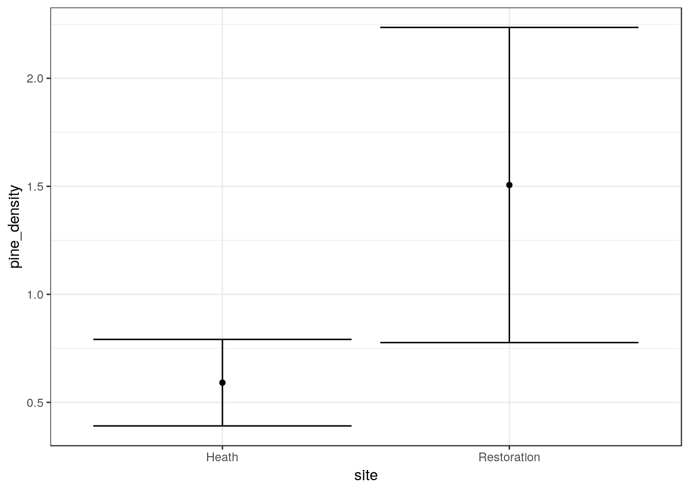
You can add labels and customize this plot in other ways. See the handout on ggplots. You should label the axes and caption the figure with an explanation of how confidence intervals have been calculated.
20.2.9 Action
- Write your own interpretation of the figure.
- Run an appropriate statistical test. (Hint .. there is a traditional and widely used test that finds the statistical significance of a difference between two means)
- What is being assumed by this test? Are these assumptions reasonable?
t.test(quadrats_2019$pine_density~quadrats_2019$site)##
## Welch Two Sample t-test
##
## data: quadrats_2019$pine_density by quadrats_2019$site
## t = -2.6065, df = 15.122, p-value = 0.01974
## alternative hypothesis: true difference in means is not equal to 0
## 95 percent confidence interval:
## -1.6627076 -0.1672924
## sample estimates:
## mean in group Heath mean in group Restoration
## 0.5911429 1.506142920.3 ——————————————————-
20.4 Investigating factors affecting pine densities on the heathland site
The assignment instructions ask you to look at whether the density of pine regeneration on the heathland is associated with elements such as slope, topographic wetness, direct beam insolation and distance to potential seed source.
To do this we first need to filter out only the quadrats that are on the heathland site.
quadrats %>% filter(site=="Heath" ) -> heath_quadratsThe coordinates are in latitude and longitude, However the Lidar data that we are going to combine with these data is held in British national grid. So we need to transform the quadrat data.
heath_quadrats<-st_transform(heath_quadrats,crs=27700)Note that the EPSG code is 27700.
20.5 Spatial data
The raster layers for Arne and some other data are bundled in a data object in the aqm package. The line below loads the data into memory.
data(arne_lidar)Notice that after running this line of code you will see some lidar derived raste layers appear in the Envir0nment panel.
- dtm The lidar derived digital terrain model at 2m resolution.
- dsm The lidar derived digital elevation model at 2m resolution.
There are many ways of making quick static maps in R from raster data. One possibility is to use qtm in the tmap package. Contours can be derived from thh dtm with one line.
contours<-rasterToContour(dtm, levels=seq(0,60,5))The results can be turned into a quick default printable map with the qtm function.
qtm(dtm) + qtm(contours) +qtm(quadrats)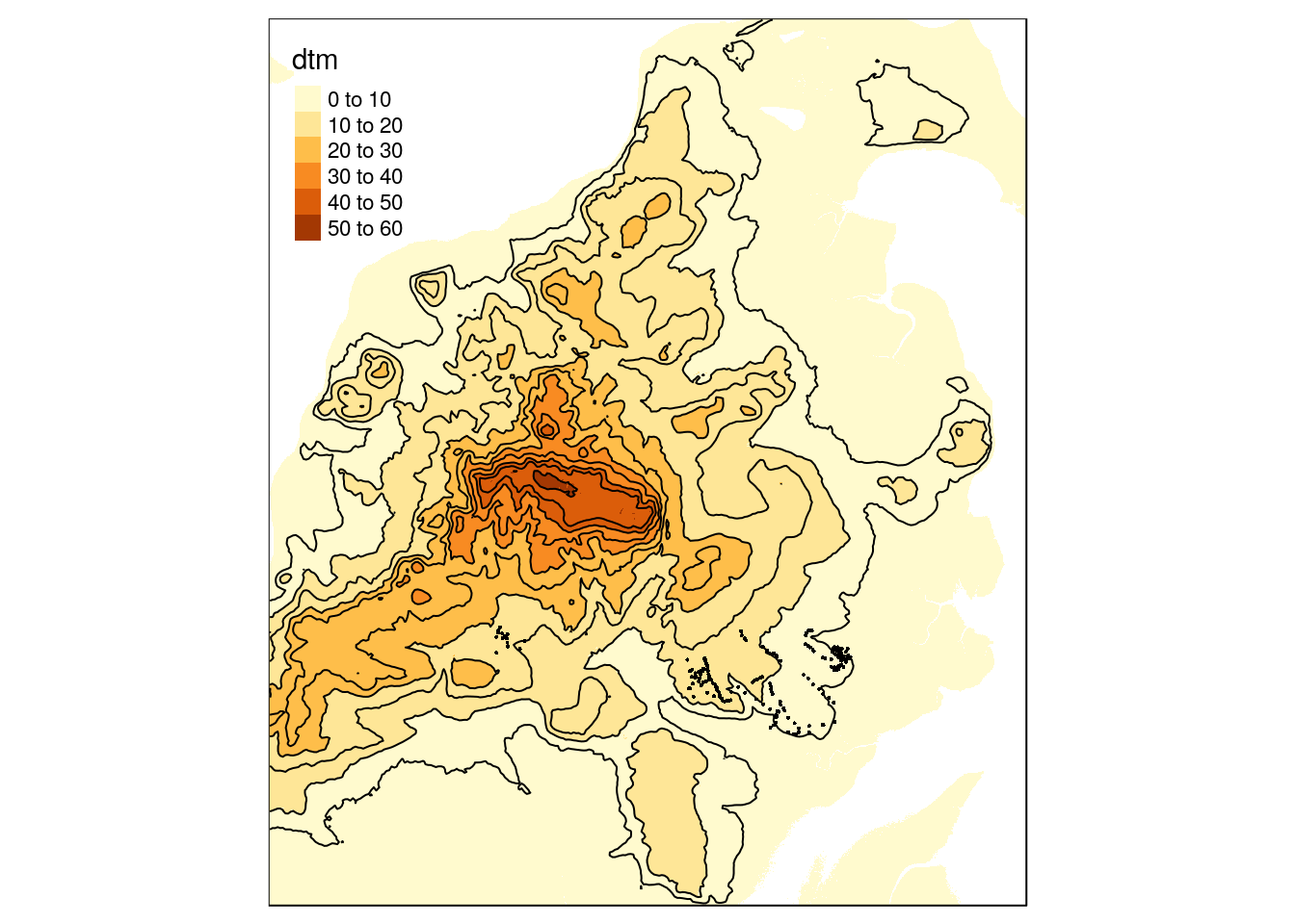
The data included a polygon drawn around the study are.
mapview(study_area,alpha.regions = 0,lwd=4) 20.5.1 Cropping
A very common GIS operation is to crop a large raster layer to the bounding box of a smaller area. This is very easy in R. We can use the study area polygon for cropping.
pol<-as(study_area,"Spatial") ## Convert to the older spatial classes
dsm<-raster::crop(dsm,pol)
dtm<-raster::crop(dtm,pol)
We can now build a mapview to look at the cropped dsm and dtm quite easily. The default colours don’t look very good, so the code also includes a palette.
contours<-rasterToContour(dtm, nlevels=10)

map2<- mapview(dsm,col.regions=terrain.colors(1000),legend=TRUE) + mapview(dtm,col.regions=terrain.colors(1000)) + mapview(contours) + mapview(heath_quadrats)

map2 %>% extras()
20.5.2 Terrain analysis
There are a large number of algorithms built into R that can be used to conduct terrain analysis. These produce the same results as the comparable options in QGIS. Working in R has the advantage of being quicker once a script has been built, and also reproducible. For example deriving slope and aspect in degrees involve running the following lines.
slope<-terrain(dtm, opt='slope', unit='degrees')
aspect<-terrain(dtm, opt='aspect',unit='degrees')
Notice that when these lines of code are run the results aren’t immediately apparent. New objects appear in the Envoronment pane. You need to plot them out are use mapview to see the results directly.
plot(slope)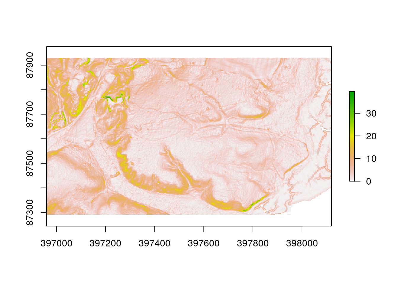
plot(aspect)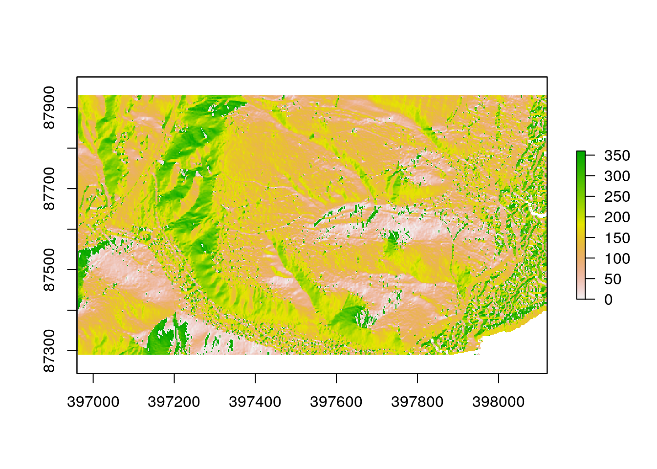
Making a hillshade layer requires slope and aspect to be calculated in radians, rather than degrees.
sloper<-terrain(dtm, opt='slope', unit='radians')
aspectr<-terrain(dtm, opt='aspect',unit='radians')
hillshade<-hillShade(sloper,aspectr,angle=5)plot(hillshade,col=grey.colors(1000),legend=FALSE) 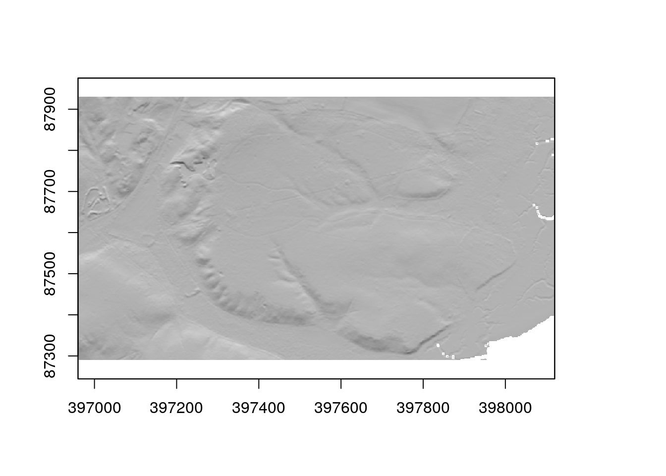
The dtm can be draped over the plot by making it semi transparent by setting an alpha level.
plot(hillshade,col=grey.colors(1000),legend=FALSE)
plot(dtm, add=TRUE, col=terrain.colors(1000),alpha=0.4)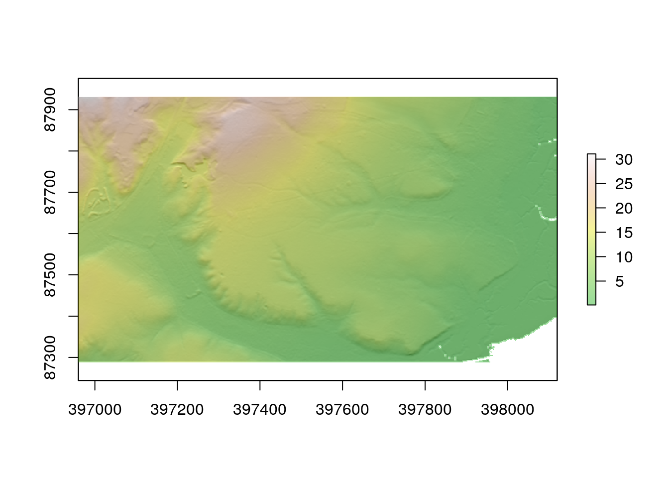
R can also call some more advanced algorithms, such as those which calculate topographic wetness index and insolation. These algorithms effectively combine elements such as slope and aspect into more interpretable variables.
twi<-giscourse::twi(dtm)
sol<- giscourse::insol(dtm, day = "11/06/2019")
The topographic wetness index measures the upslope area draining through a certain point per unit contour length. In other words values of the topographic wetmess index (which is unitless) can be used to compare where a quadrat lies on a slope. Water drains from low values to high values, so on average the soil will be moister although we may not know by how much) when the index is low.
plot(twi)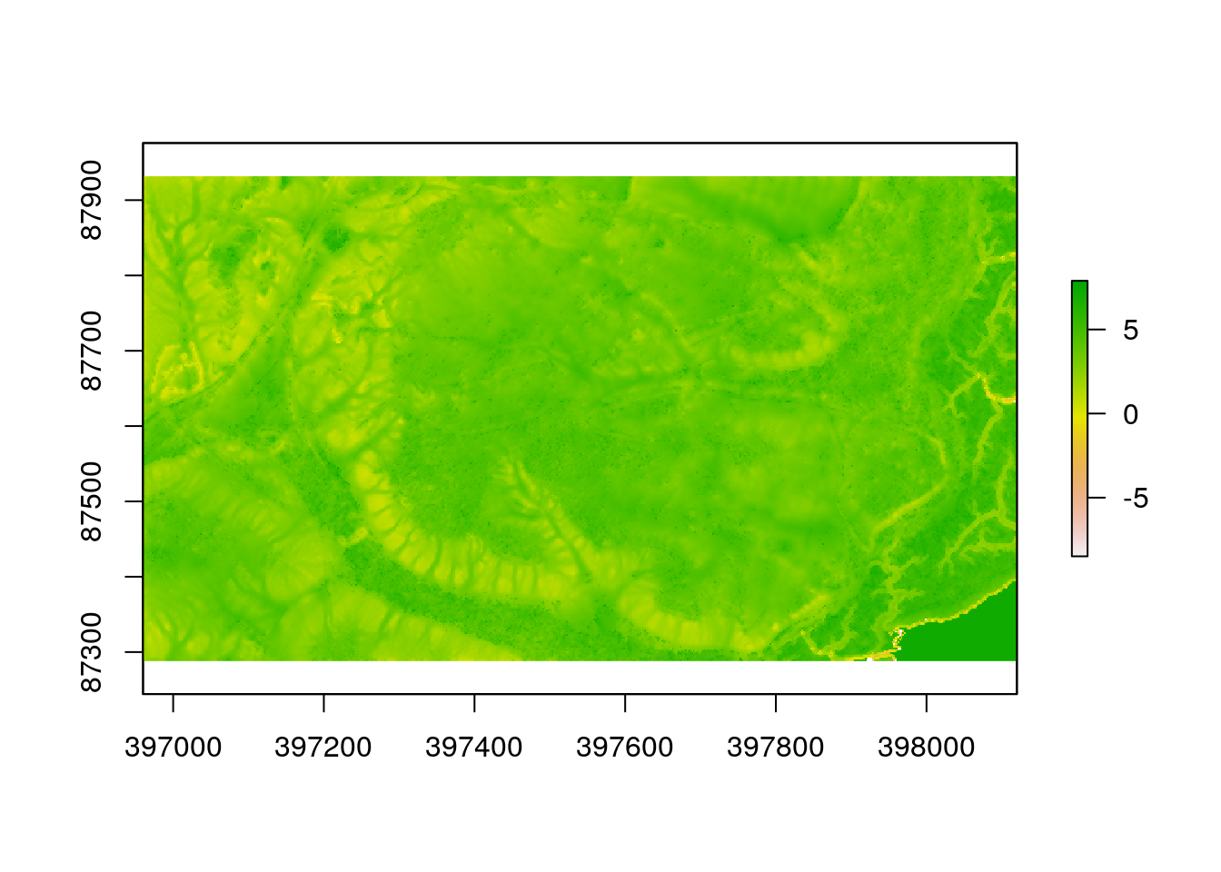
The insolation layer is caluculated precisely using mechanistic preinciples. When a date is provided for the algorithm the routine steps through each hour of the day and calculates the solar energy that each pixel will recieve on a totally clear day through direct beam insolation. All other things being equal, pixels with high values will warm up more than pixels with low values on a sunny day. The pattern will change over the year.
plot(sol)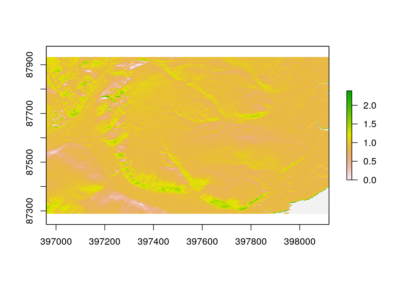
20.6 Raster algebra
Carrying out raster algebra (i.e. sums) operations in R is very simple and inuitive. To obtain the height of vegetation (and maybe some buildings ) we just need to subract the digital terrain model from the digital surface model.
chm<-dsm-dtm
plot(chm)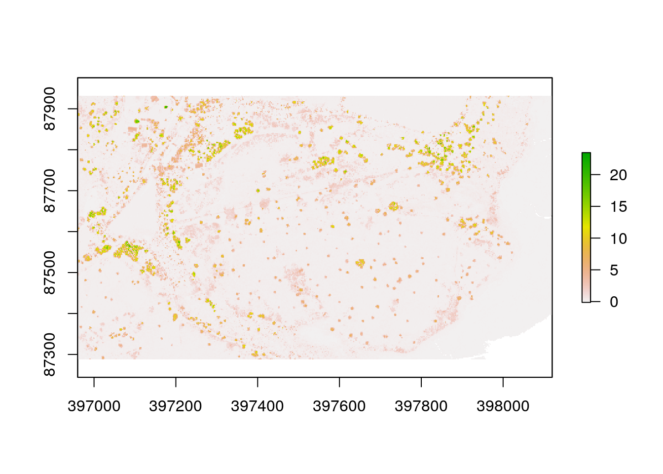
20.7 Raster aggregation
We often need to coarsen the resolution of a raster map and use some statistic calculated from all the pixels within a window. For example, if we are interested in the vegetation height around a study point we would not want to know the precices height at the point as it might just happen to fall into a small gap in a forest canopy. The orginal raster is at 2m resolution, so if we want mean vegetation height at 10m resolution we use factor of 5.
chm10<-aggregate(chm, fact=5, fun=mean, expand=TRUE, na.rm=TRUE)We may want to set all values below a low threshold to NA
chm[chm<0.1]<-NA
chm10[chm10<0.2]<-NAmapview(chm10,col.regions=terrain.colors(100)) -> map3
map3 %>% extras()20.7.1 Action
Investigate this map. Compare the canopy height model with the Esri satelite image. Does the canopy height model reliably pick out trees and taller vegetation?
20.8 Adding the values to the quadrats
IN the context of the assignment the reason for producing the raster maps is to find the values for the variables that coincide with the quadrats that we placed on the ground. This is like placing your finger on each of the maps at the position of the quadrat, reading off the value, then adding the value to the original spreadheet of results. Rather than go through this very tedious process we can run some lines of R code to do the same.
hq<-as(heath_quadrats,"Spatial")

heath_quadrats$twi<-raster::extract(twi,hq)
heath_quadrats$sol<-raster::extract(sol,hq)
heath_quadrats$dtm<-raster::extract(dtm,hq)
heath_quadrats$slope<-raster::extract(slope,hq)
20.9 Distances to trees
To calculate the distance between the quadrats and the nearest tree we can use the canpoy height model. Assuming that the heights represent vegetation we can first make polygons that represent groups of pixels over a given height.
chm[chm<2]<-NA ## Set below 2m as blanks (NA)
chm[chm>=2]<-1 ## Set above 2m to a single value
trees<-rasterToPolygons(chm, dissolve=TRUE)
trees<-st_as_sf(trees)
st_crs(trees)<-27700
trees<-st_cast(trees$geometry,"POLYGON")
map1 + mapview(trees)Now once we have the objects that represent the “trees” we can make a distance matrix. This contains all the distances measured between the quadrats and the trees.
distances<-st_distance(heath_quadrats,trees)
dim(distances)
## [1] 184 1666Finally to calculate the distances, find the minimum between each quadrat and the trees.
heath_quadrats$min_dist<-apply(distances,1,min)Now we can check if the distances are right by using the measuring tool
mapview(heath_quadrats, zcol='min_dist') + mapview(trees) ->map4
map4 %>% extras()
20.10 Data table
The resulting data table can be written out as a data frame. This can form the basis of your statistical analysis. See the next handout.
heath_quadrats %>% st_set_geometry(NULL) -> quads
  dt(quads)
20.11 Writing out the data
The resulting data table can be written out as a data frame. This can form the basis of your statistical analysis. See the next handout.
write.csv(quads, file="arne_quadrats.csv", row.names=FALSE)
#arne_quads <-quads
#save(arne_quads,file="~/rstudio/aqm/data/arne_quads.rda")