Chapter 14 Crib sheet for GIS in R

14.1 Introduction

The code assumes that the GIS layers exist in a folder called gis_data, which has a path to it on the folder as defined below. Otherwise It won’t actually run. However the code chunks can be adapted to other data sources easily enough.

library(sp)
library(raster)
library(rgeos)
library(rgdal)
library(RColorBrewer)
library(leaflet.extras)
library(mapview)
library(sf)
path<-"/home/rstudio/webpages/Quantitative_and_Spatial_Analysis/Quantitative_and_Spatial_2018/Arne_project/gis_data"

14.2 Reading in a shapefile

This uses the sf package. You need to provide the path to the directory and the name of the shapefile, without extension. Remember that a “shapefile” actually consists of four files. You need all to be present in the folder.

polys<-read_sf(path,"sssi")

14.3 Transforming to British National Grid

The EPSG code for British national grid is 27700. If your shapefile is in another CRS you may need to transform it.

polys<-st_transform(polys,27700)
st_crs(polys) ## CHeck the CRS

## Coordinate Reference System:
##   EPSG: 27700 
##   proj4string: "+proj=tmerc +lat_0=49 +lon_0=-2 +k=0.9996012717 +x_0=400000 +y_0=-100000 +ellps=airy +towgs84=446.448,-125.157,542.06,0.15,0.247,0.842,-20.489 +units=m +no_defs"

14.4 Mapview of a polygon layer

If you want to change the order of the basemaps or add more options change this chunk, that you run before making any maps.

mapviewOptions(basemaps =c("OpenStreetMap","Esri.WorldImagery",  "OpenTopoMap", "OpenStreetMap.BlackAndWhite", "OpenStreetMap.HOT"))

You can find more named basemaps from here.

http://leaflet-extras.github.io/leaflet-providers/preview/

In this particular shapefile there is a column for id. That’s not very interesting, but we can shade on it.

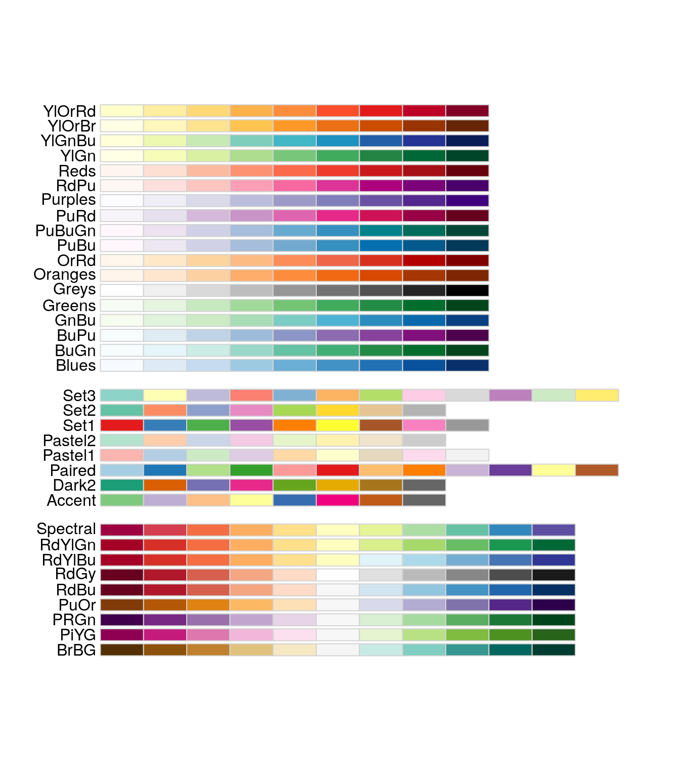
You can find a palette from here. http://colorbrewer2.org

Or use this chart

library(RColorBrewer)
display.brewer.all()

Set the number of levels and find the code letters for the palette and change the line used to make the pal object.

Set the alpha variable to a number between 0 (invisible) and 100 (opaque)

pal<-brewer.pal(9, "Set1")

alpha=100

mp<-mapview(polys, zcol = "id",col=pal, col.regions = pal,legend = TRUE,alpha.regions=alpha/100)

mp

14.5 Adding an overview map

The code above forms a map object that can be modified through adding components. It is a good idea to add a full screen control. A mini map provides an overview. You can change the tile and zoom level. The best position is usually the bottomleft.

tile<-"CartoDB.Positron" ## Change if needed
zoom<- - 4  ## Larger negative values to zoom out
pos<-"bottomleft"

mp@map %>% addFullscreenControl() %>%
  addMiniMap(position=pos,zoomLevelOffset = zoom,tiles=tile) 

14.6 Adding a measurement tool

mp@map %>% addFullscreenControl() %>%
  addMeasurePathToolbar() %>%
  addMeasure( primaryLengthUnit = "meters", primaryAreaUnit = "hectares")

 #

14.7 Reading in points from a CSV

Point data often is provided as a simple table with X and Y coordinates. This can be easily conversted to a spatial object, However you must know the CSV.

pnts<-read.csv(paste(path,"study_points.csv",sep="/"))

#coordinates(pnts) = ~X+Y  # Set coordinates
#pnts<-st_as_sf(pnts)  # Make sf object
#st_crs(pnts) <-27700 ## Set CRS


pnts<-st_as_sf(pnts, coords = c("X", "Y"), crs = 27700) ## Better way

The points can then be plotted as a mapview. The col.region setting determines the fill color.

If the points are in fact in latitude and longitude then declare this, and if necessary transform.

#st_crs(pnts) <-4326 
#pnts<-st_transform(pnts, 27700)

Mapview maps are additive. so the points can be placed on the previously saved map. T

mp<-mp + mapview(pnts,col.regions="red")  ## mp was built above

mp@map %>% addFullscreenControl() %>%
  addMiniMap(position=pos,zoomLevelOffset = zoom,tiles=tile) 

Note that one slightly annoying feature of mapview is that legends do not disappear when a layer is not selected. So be careful when adding maps together. For clarity it may be preferable to make separate maps when using them to illustrate some aspect of the study as a static figure.

A column can also be used to shade points with a legend as was used for the polygons.

pal<-brewer.pal(11, "YlOrBr")

mapview(pnts, zcol = "npines",col.regions=pal,legend=TRUE)

14.8 Reading raster data

slope<-raster(paste(path,"slope.tif",sep="/"))
aspect<-raster(paste(path,"aspect.tif",sep="/"))
dtm<-raster(paste(path,"dtm.tif",sep="/"))

14.9 Making colour ramps for raster data

Displaying raster data can be quite challenging, as you need to find a good colour scheme. You may be able to use the brewer palettes, but they need to be turned into a ramp using an extra line of code. Some trial and error may be needed to find a suitable colour mix.

pal<-brewer.pal(11, "PuOr")
pal <- colorRampPalette(pal)


mapview(aspect,col.regions=pal, legend=TRUE)

There are also some pre built palettes in R. The terrain colours can be useful.

pal<-terrain.colors(100)

pal <- colorRampPalette(pal)
mapview(dtm,col.regions=pal, legend=TRUE)

As previously, you can add elements such as a minimap and a full screen control to raster maps.

mp<-mapview(dtm,col.regions=pal, legend=TRUE)
mp@map %>% addFullscreenControl() %>%
  addMiniMap(position=pos,zoomLevelOffset = zoom,tiles=tile) 

14.10 Extracting raster values for points

There are some complex elements involved in spatial overlays.

However the simplest idea of taking the values from a raster layer and adding them to a data frame of points is very straightforward. Simple feature layers need to be transformed to the older spatial class in R. The following lines adds aspect derived from the raster layer to the points object.

pnts<-as(pnts, "Spatial")
pnts$aspect<-raster::extract(aspect,pnts)
pnts<-st_as_sf(pnts)