Chapter 19 Analysing the residuals from regression analysis on individual pines from the Arne 2019 data
19.1 Introduction
In today’s class you will learn how to run a regression analysis in R using the data collected from Arne as an example.
There are several handouts in both the online course book for this unit and AQM that cover the theory of regression in more depth. The purpose of this class is to provide the tools in R to run a regression and interpret the output.
19.1.1 Load R libraries
The libraries that are almost always used in any R analysis include ggplot2 (for graphics) dplyr (for data manipulation) and readr/readxl for data import.
library(ggplot2)
library(aqm)
library(dplyr)
library(mgcv)

library(mapview)
library(sf)
19.1.2 Load the data
When the data is loaded from the aqm package it also contains the gps way points that you collected.
## This loads data from the aqm package
data(arne_2019)mapview(gps)You can look at the points as a data frame
gps %>% st_set_geometry(NULL) %>% dt()Notice that the waypoints alone do not contain a variable that indicates the site.
One way to obtain this (there are a lot of possibilities) is to cluster the points by proxmity.
clust<-hclust(dist(st_coordinates(gps)))  ## Default option for a distance matrix uses euclidaen distance which is what we want.
plot(clust)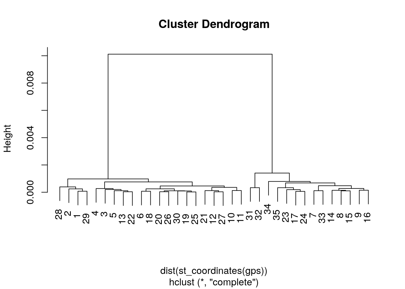
There are clearly two main clusters of points.
The cutree function in R cuts this tree into a given number of groups and returns an identifying number for the group. So we can now find the two sites easily and map the results out.
gps$site<-as.factor(cutree(clust,2))
mapview(gps,zcol="site", burst=TRUE)
19.2 Adding the GPS points to the pines
When we have two different data tables in R of any type we can always join them together if we can find a unique identifying feature that the two data sets have in common.
Let’s look at the names of the variables in the gps data
str(gps)## Classes 'sf' and 'data.frame': 35 obs. of 5 variables:
## $ name : Factor w/ 11 levels "001","002","003",..: 1 2 3 4 5 6 7 8 9 1 ...
## $ time : POSIXct, format: "2019-10-30 11:35:43" "2019-10-30 11:55:18" ...
## $ group : Factor w/ 4 levels "A","B","C","D": 4 4 4 4 4 4 4 4 4 1 ...
## $ geometry:sfc_POINT of length 35; first list element: 'XY' num -2.04 50.69
## $ site : Factor w/ 2 levels "1","2": 1 1 1 1 1 1 2 2 2 1 ...
## - attr(*, "sf_column")= chr "geometry"
## - attr(*, "agr")= Factor w/ 3 levels "constant","aggregate",..: NA NA NA NA
## ..- attr(*, "names")= chr "name" "time" "group" "site"The element that uniquely identifies the point is the name of the waypoint combined with the group that collected the data.
The pine_hts data has similar fields.
str(pine_hts)## Classes 'tbl_df', 'tbl' and 'data.frame': 256 obs. of 6 variables:
## $ Group: chr "A" "A" "A" "A" ...
## $ Site : num NA NA NA NA NA NA NA NA NA NA ...
## $ WP : num 1 1 1 2 2 2 3 3 3 4 ...
## $ Age : num 8 4 7 5 7 7 4 5 4 5 ...
## $ DiMM : num 26.77 6.39 14.41 35 25.65 ...
## $ HeCM : num 100 43 72 125 95 77 95 99 75 141 ...Notice that the Site column is currently blank. We can make an id column for each set of data, then merge the results.
gps$id<-paste(gps$group,as.numeric(gps$name), sep="_")
pine_hts$id<-paste(pine_hts$Group,pine_hts$WP, sep="_")
pine_hts_gps<-merge(gps,pine_hts)mapview(pine_hts_gps,zcol="site")19.3 Looking at the residual
Let’s make a working data frame to simplify typing.
d<-pine_hts_gpsThese data are the same as we used previously, so the scatterplot should look the same.
fig1<-ggplot(d,aes(x=DiMM, y=HeCM)) +geom_point() + geom_smooth()
fig1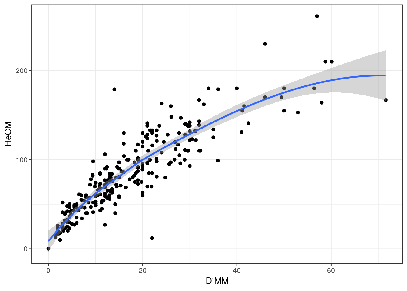
19.3.1 Plotting the data by site
If we add a colour aesthetic to our ggplot then the data will be split into two labeled groups which correspond with the site.
fig2<-ggplot(d,aes(x=DiMM, y=HeCM, colour=site)) +geom_point() + geom_smooth()
fig2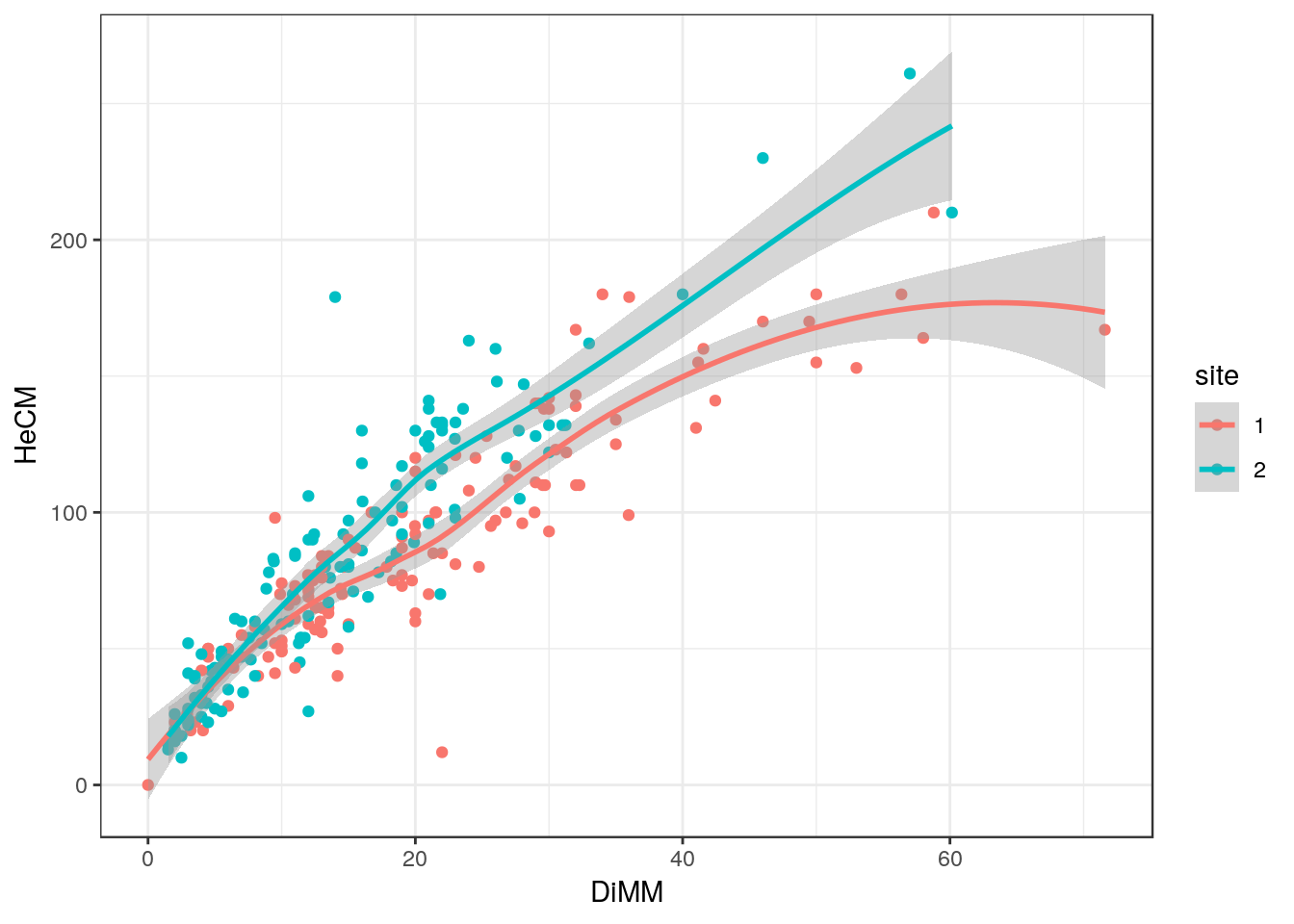
What can you see from this figure?
19.3.2 Obtaining residuals
Last time we tried fitting both lines and splines to the height diameter relationship. Regression lines were found to be useful for summarising the reslationship, but splines provided a closer fit to the actual data. So we can take the residuals from the spline.
d$residuals<-residuals(gam(data=d,HeCM~s(DiMM)))This is the equivalent of measuring the distance between the fitted line shown in figure one and each data point. Some will be positive and others negative. Negative values imply that the pine height is lower than expected for a given diameter.
19.3.3 Plotting the residuals by site
fig3<-ggplot(d,aes(x=site,y=residuals))
fig3 + geom_boxplot()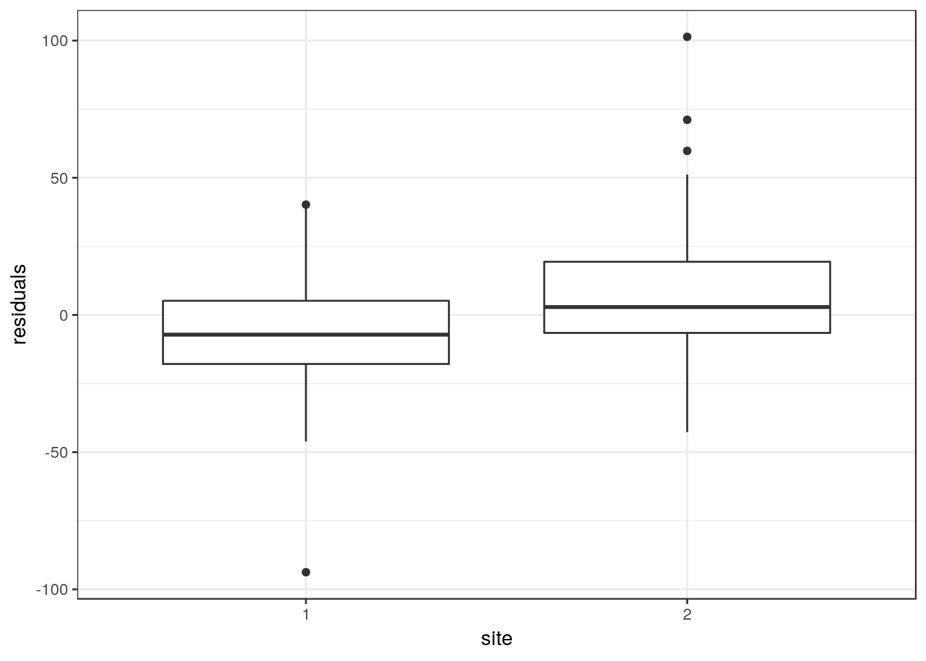
19.3.4 Confidence intervals
aqm::ci(fig3)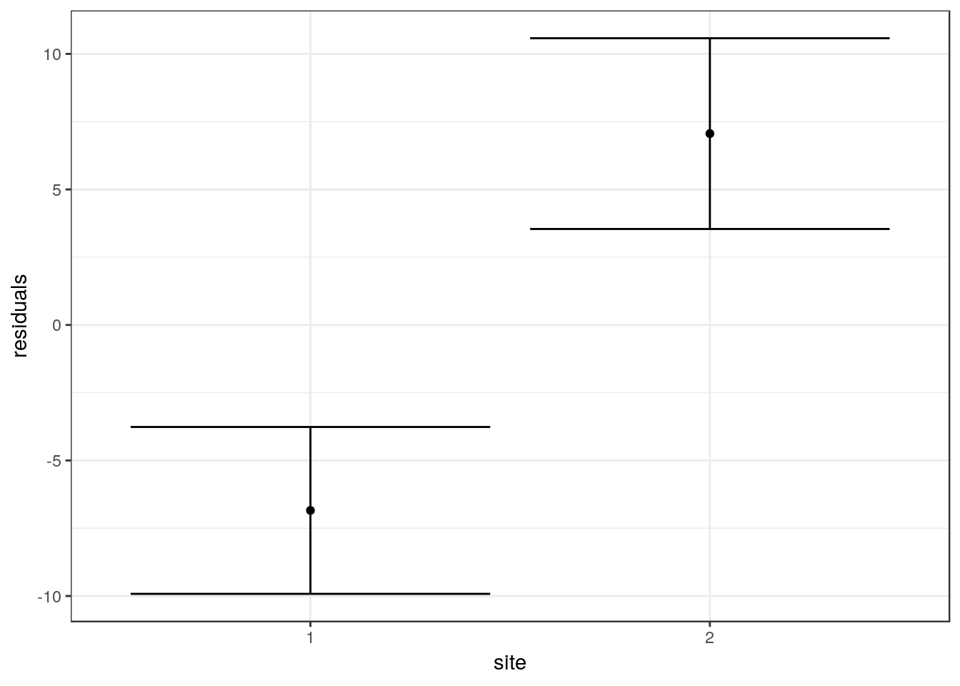
19.3.5 Simple unpaired t-test
t.test(d$residuals~d$site)##
## Welch Two Sample t-test
##
## data: d$residuals by d$site
## t = -5.884, df = 248.55, p-value = 1.289e-08
## alternative hypothesis: true difference in means is not equal to 0
## 95 percent confidence interval:
## -18.556135 -9.248877
## sample estimates:
## mean in group 1 mean in group 2
## -6.842640 7.059866