Chapter 14 Brief introduction to analysis of covariance
library(tidyverse)
library(multcomp)
library(aqm)
This type of analysis is not needed to complete the assignment as set. However, it could come in useful for some of the possible questions that could be addressed using the data set. The specific relationships shown below are rather trivial, but others may possibly be more interesting. Do not try to use this technique unless you really feel that it is useful and you understand the basic idea. If not, you can ignore this section for this particular unit. We will return to the theme in AQM, as it is rather advanced.
Analysis of covariance is a handy technique to know about. The full details around use of the technique and the theory behind it is rather complex, and it can be applied in a variety of ways. However the most common reason to apply analysis of covariance to an observational data set is quite straightforward.
If we can assume that there exists a simple linear relationship between two numerical variables, we might ask if this relationship varies between levels of a categorical variable.
Let’s take the sleep data set as an example.
data("sleep")
d<-sleep
d$logBodyWt<-log10(d$BodyWt)
d$logBrainWt<-log10(d$BrainWt)
We can easily show that there is a (trivially) strong relationship between logBrainWt and LogBodyWt. This is well modelled by regression.
g0<-ggplot(data=d,aes(x=logBodyWt,y=logBrainWt))
g1 <- g0 + geom_point() + geom_smooth(method="lm")
g1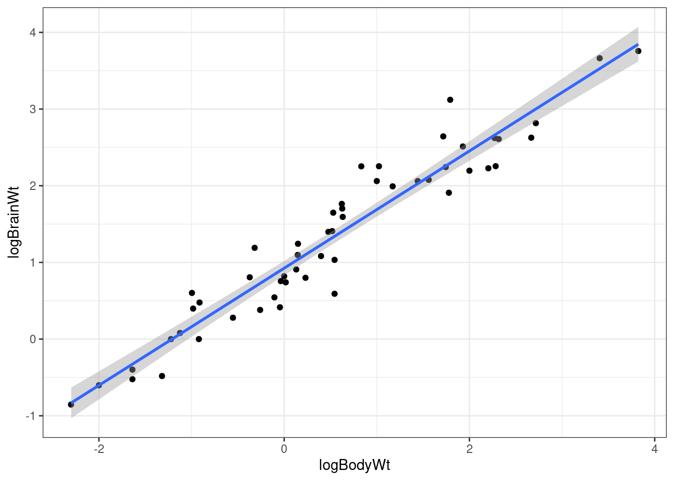
We have already seen that the residuals can be taken from the fitted model and used in a subsequent analysis.
However, we might ask if the same relationship holds for each level of diet. Let’s plot this out and look at it.
g0<-ggplot(data=d,aes(x=logBodyWt,y=logBrainWt, col=Diet))
g1 <- g0 + geom_point() + geom_smooth(method="lm")
g1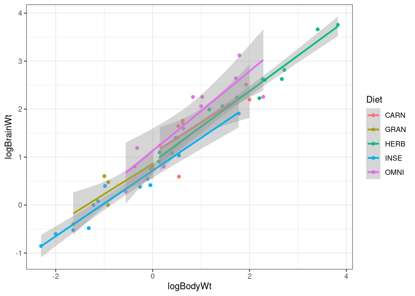
It looks as if the slopes of the lines are actually very similar. A test of this consists of fitting a model with an interaction between logBodyWt and Diet. If the interaction is significant then there is an indication of variability between the slopes of the lines.
mod<-lm(data=d,logBrainWt~logBodyWt*Diet)
anova(mod)
## Analysis of Variance Table
##
## Response: logBrainWt
## Df Sum Sq Mean Sq F value Pr(>F)
## logBodyWt 1 58.934 58.934 669.0647 < 2e-16 ***
## Diet 4 1.172 0.293 3.3270 0.01846 *
## logBodyWt:Diet 4 0.159 0.040 0.4506 0.77138
## Residuals 43 3.788 0.088
## ---
## Signif. codes: 0 '***' 0.001 '**' 0.01 '*' 0.05 '.' 0.1 ' ' 1In this case the interaction is not significant F(4,43)=0.4, p= 0.8. So we could stop at this point and conclude that there is no detectable difference between the slopes. The (weakly) significant effect of diet implies that there may be a difference between logbrainweights that is attributable to diet after accounting for the effect of logBodyWt. This could be investigated more simply by taking the residuals from the overall relationship for all the species.
If the interaction had been significant then things would get a little more complex, as we may wish to carry out specific comparisons.
# Use filter to select two of the levels
d %>% filter(Diet %in% c("HERB","CARN")) -> d1

g0<-ggplot(data=d1,aes(x=logBodyWt,y=logBrainWt, col=Diet))
g1 <- g0 + geom_point() + geom_smooth(method="lm")
g1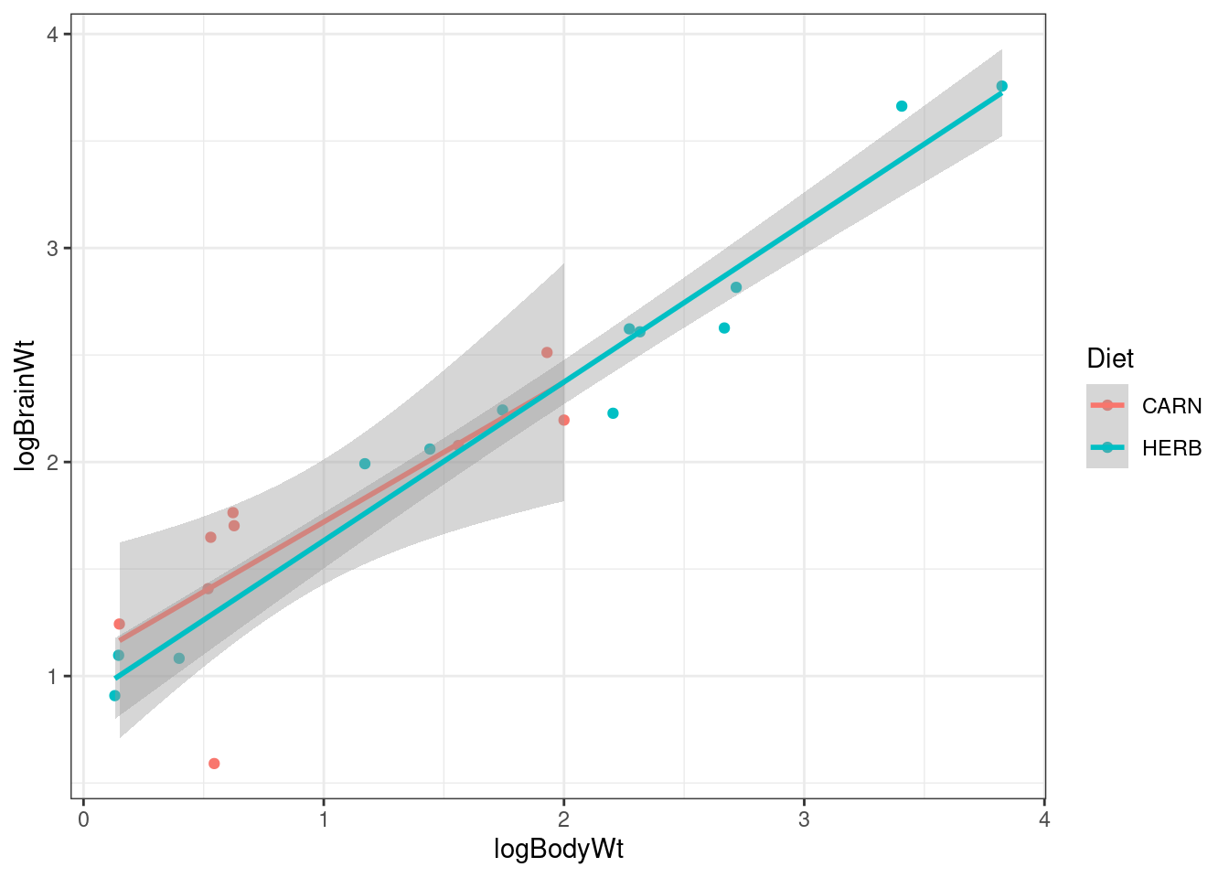
We have already seen that the overall model did not detect a difference, so when we fit a model to the subset of the data and obtain a confidence interval for the difference between the two slopes we would expect it to include zero.
mod<-lm(data=d1,logBrainWt~logBodyWt*Diet)
confint(mod)
## 2.5 % 97.5 %
## (Intercept) 0.7412456 1.3949104
## logBodyWt 0.3666209 0.9373737
## DietHERB -0.6192646 0.2658567
## logBodyWt:DietHERB -0.2266516 0.4054096Which it does.
There is more to learn about this technique in order to fully appreciate the subtleties involved, but this introduction is enough to allow you to ask (and answer) questions involving differences between the slopes of responses.
14.1 Mussels example
The same sort of (non significant) findings apply to the mussels data.
data(mussels)
d<- musselsg0<-ggplot(data=d,aes(x=Lshell,y=BTVolume, col=Site))
g1 <- g0 + geom_point() + geom_smooth(method="lm")
g1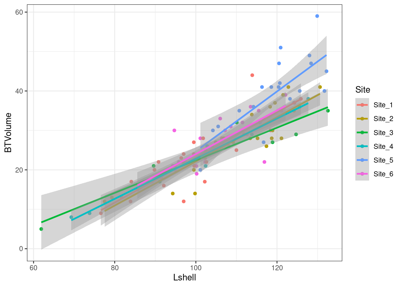
mod<-lm(data=d,BTVolume~Lshell*Site)
anova(mod)
## Analysis of Variance Table
##
## Response: BTVolume
## Df Sum Sq Mean Sq F value Pr(>F)
## Lshell 1 8811.4 8811.4 468.3859 < 2.2e-16 ***
## Site 5 578.4 115.7 6.1496 5.144e-05 ***
## Lshell:Site 5 147.3 29.5 1.5658 0.1766
## Residuals 101 1900.0 18.8
## ---
## Signif. codes: 0 '***' 0.001 '**' 0.01 '*' 0.05 '.' 0.1 ' ' 1You might think from the first figure that there could be a difference in slopes between site 1 and site 5. However the overall test has not shown any significant variability so a specific comparison should reach the same conclusion.
d %>% filter(Site %in% c("Site_1","Site_5")) ->  d1
g0<-ggplot(data=d1,aes(x=Lshell,y=BTVolume, col=Site))
g1 <- g0 + geom_point() + geom_smooth(method="lm")
g1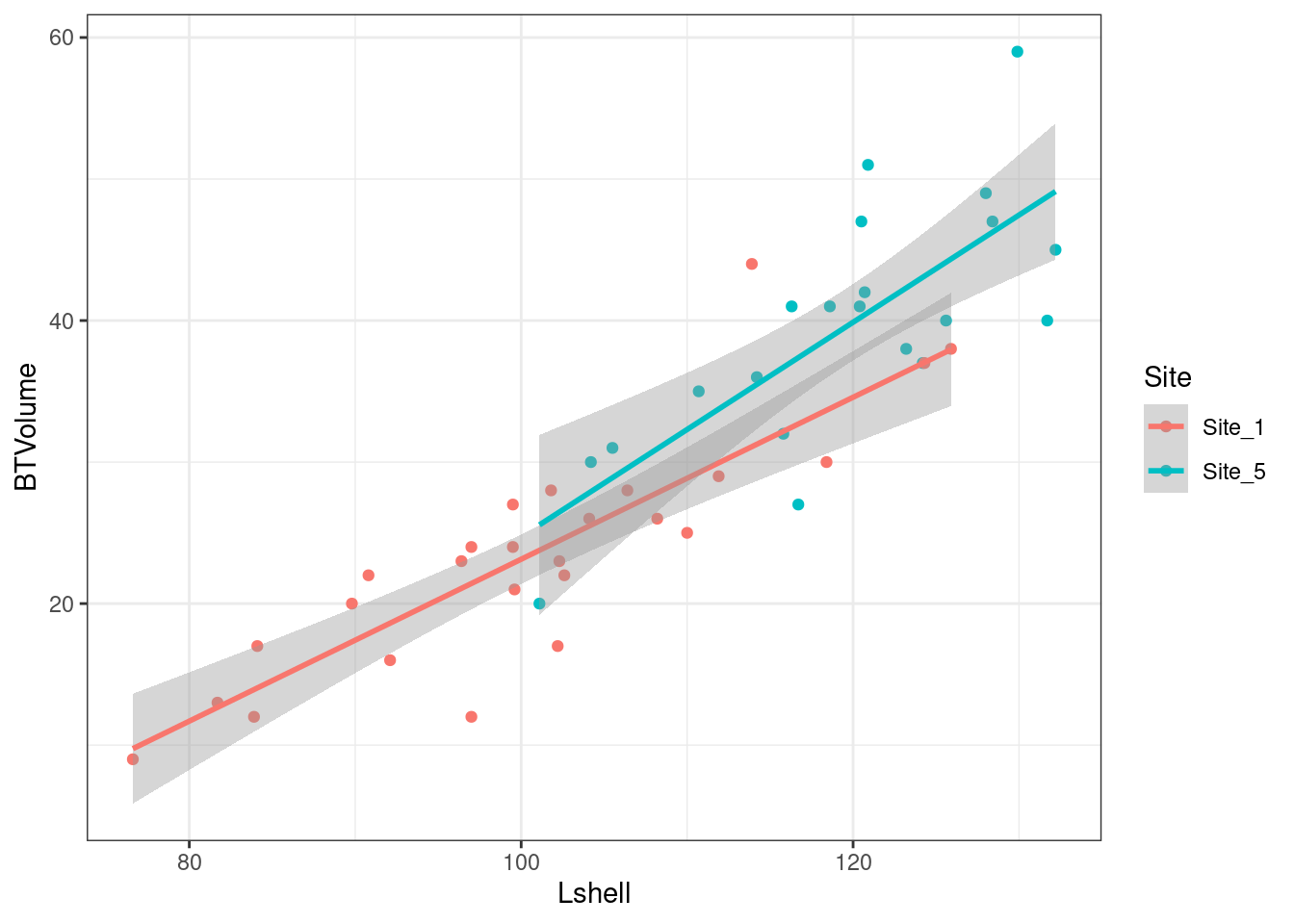
mod<-lm(data=d1,BTVolume~Lshell*Site)
anova(mod)
## Analysis of Variance Table
##
## Response: BTVolume
## Df Sum Sq Mean Sq F value Pr(>F)
## Lshell 1 4931.2 4931.2 191.4060 < 2e-16 ***
## Site 1 117.1 117.1 4.5449 0.03877 *
## Lshell:Site 1 38.1 38.1 1.4780 0.23072
## Residuals 43 1107.8 25.8
## ---
## Signif. codes: 0 '***' 0.001 '**' 0.01 '*' 0.05 '.' 0.1 ' ' 1mod<-lm(data=d1,BTVolume~Lshell*Site)
confint(mod)## 2.5 % 97.5 %
## (Intercept) -50.8379073 -17.3122499
## Lshell 0.4069676 0.7372706
## SiteSite_5 -52.2822444 18.3684719
## Lshell:SiteSite_5 -0.1222044 0.4931697As always the caveats regarding statistical signficance apply. You have not shown that there is no difference. The analysis fails to detect a difference, given the sample used.