Chapter 19 Arne pine density: Spatial data
library(tidyverse)
library(aqm)
library(giscourse)
library(sf)
library(mapview)
library(raster)
library(leaflet.extras)
library(RColorBrewer)
pal1<-terrain.colors(100)
pal2<-gray(0:100 / 100)
19.1 Introduction
In the last chapter we have looked at how a simple set of data collected fairly quickly can be used to estimate the number of regenerating pine trees on Grip heath. However there are many challenges regarding the representativeness of the samples taken. These should be discussed with reference to the spatial pattern shown on the maps and the issue of changes to the numbers of pines over time as a result of management.
It is possible that the density of regenerating pines could be related to topographic features of the site. In order to look at this we can use digital terrain models and digital surface models derived from lidar data.
19.2 Obtaining Lidar data
The repository for openly available lidar data online has changed several times in the last few years. The most comprehensive source is now held by DEFRA.
https://environment.data.gov.uk/DefraDataDownload/?Mode=survey
Downloading the data is fairly straightforward, but is still something of a hassle for use in class.The DEFRA interface can produce a large number of files for a single site. You should be aware that this data is available and can be imported into R if you are working at a specific site for your own project, but for the purposes of this unit we will use data that is already loaded. This data is a little out of date, but corresponds to the situation when the field data was collected.

19.3 Loading the lidar data
The following line loads the saved Lidar derived 2m DTM and DSM layers for the Arne area together with a polygon representing the study site.
data(arne_lidar)
study_area<-st_transform(study_area,27700)
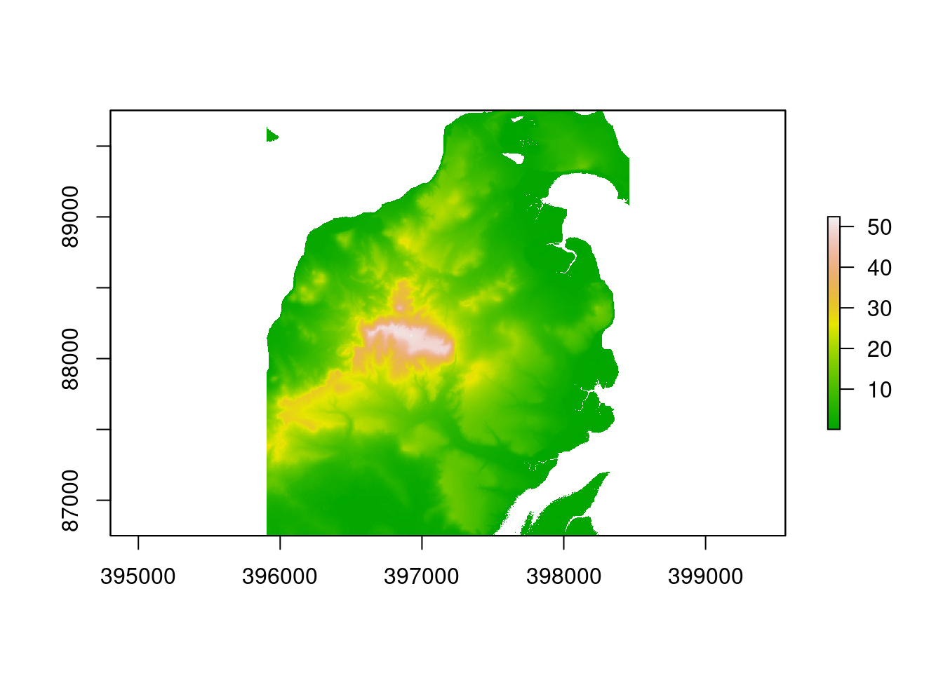
A quick plot of the dtm shows the layer.
plot(dtm, col=pal1)
19.3.1 Exercise
Use the code from the terrain analysis class to produce a shaded hill layer for Arne and display this as a map.
19.4 Cropping and masking to the study site
The code also loaded a polygon representing the heathland study area. A sing
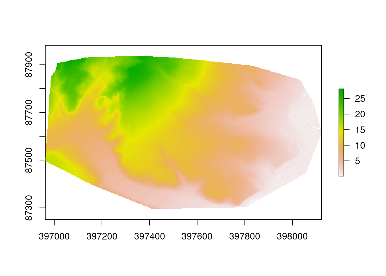
dtms<-crop(dtm, study_area)
dtms<-mask(dtms, study_area)
plot(dtms)
19.4.1 Exercise
1.Crop and mask the DSM
Derive a canopy height model for the study are and plot it. A canopy height model is the difference between the DSM and DTM. It can be found by a simple map algebra operation.
Play around with the maps you have. Try deriving slope aspect and hillshades and plotting them out using code from the last class.
19.5 Reloading the quadrats
The code below reloads the data from the last chapter and converts it into a spatial object. Notice that the CRS is transformed to EPSG code 27700 (British National Grid) in order to match the lidar raster layers.
data("grip")
quadrats<-st_as_sf(grip,coords = c("lon","lat"),crs=4326)
d<-st_transform(quadrats,27700)
To find the elevation at any of the points we use the extract function in the raster package.
d$dtm<-raster::extract(dtms, d)Now if you look at the object you will see that the relevant values have been added. This process can be repeated for any raster layer derived from the two layers.
19.6 Forming additional data from the raster layers
The giscourse package contains a couple of functions to use the SAGA algorithms ta_hydrology and ta_lighting to extract a topographic wetness index (twi) and daily direct beam insolation from the digital terrain model.
insol<-giscourse::insol(dtms)
names(insol)<-"insol"
twi<-giscourse::twi(dtms)
names(twi)<-"twi"
slope<-terrain(dtms,"slope")
aspect<-terrain(dtms,"aspect")
19.7 Adding the values to the quadrat data
If we bundle layers together as a raster brick the extract function only needs to be run once to extract all the values and assign them to the spatial object.
lyrs<-raster::brick(insol,twi,slope,aspect)
d<-cbind(d,raster::extract(lyrs, d))str(d)## Classes 'sf' and 'data.frame': 184 obs. of 8 variables:
## $ Year : num 2019 2019 2019 2019 2019 ...
## $ pine_density: num 0.875 0.557 0.955 0.239 0.318 0.637 0.398 0.637 0.557 0.477 ...
## $ dtm : num 12.6 12.8 13 13.3 13.2 ...
## $ insol : num 1.83 1.88 1.81 1.78 1.84 ...
## $ twi : num 4.24 3.96 3.64 4.14 4.26 ...
## $ slope : num 0.0224 0.0338 0.0339 0.015 0.0213 ...
## $ aspect : num 1.57 2.15 1.98 1.38 2.13 ...
## $ geometry :sfc_POINT of length 184; first list element: 'XY' num 397381 87509
## - attr(*, "sf_column")= chr "geometry"
## - attr(*, "agr")= Factor w/ 3 levels "constant","aggregate",..: NA NA NA NA NA NA NA
## ..- attr(*, "names")= chr [1:7] "Year" "pine_density" "dtm" "insol" ...19.7.1 Finding distance from paths
The open street map layer that you can see as a basemap can also be downloaded as a vector layer. The process of doing this is a little complex, so I have done this for you and placed the data in the aqm package.
data(arne_paths)
paths<-st_intersection(paths,study_area)
mapview(paths)
Now if we want to add the distance from the path to each quadrat it is easy.
d$path_dist<-apply(st_distance(d,paths),1,min)save(d,study_area,file="arne_assignment.rda")See the next section for more detail on measuring distances.