Chapter 4 Phase 1 map example
In previous years the quantitative and spatial analysis usint has included an assignment that invoved forming a phase one map using a desktop GIS (QGIS).
Some handouts showing how to do this are available here. http://r.bournemouth.ac.uk:82/books/quant_spat/_book/on-screen-digitising.html
On screen digitising can be rather frustrating and time consuming, but in many ways it is actually easier to produce simple maps in R than in a desktop GIS. The exercise does involve a few steps, so be careful and patient the first time.
The handbook for phase 1 mapping can be found here.
I will assume that the field at the entrance to Hengistbury head has two habitat types. The habitat types themselves cannot be discerned directly from a satellite image. There is no way to know whether the grassland is acidic or basic from the imagery. So ground truthing is essential, as you found oout on the field trip. So this is for illustration of the concept.
B1.1 Unimproved acid grassland
D1.1 Dry acid heathland
Note that there is also a scaling issue involved. If the “minimum mappable area” was over one hectare then the code for the whole field could be D5 Dry heath acid grassland mosaic.
First run the following code to ensure all the libraries are loaded. Note that the mapview options set the order of the basemaps. (Since updating the package I noticed that this line was required to prevent the map occasionally dropping back to just a single layer .. I assume this is a minor bug that will be fixed later in the package, but this line prevents it happening)
library(tidyverse)
library(giscourse)
library(mapview)
mapviewOptions(basemaps =c("Esri.WorldImagery","OpenStreetMap", "CartoDB.Positron", "OpenTopoMap"))
library(tmap)
library(sf)
4.1 Digitising
Now stop looking at the markdown temporarily and switch to the console in order to digitise your map.
When digitising each polygon will be given a sequential id code beginning with 1, up to the number of polygons added. It is important to note the id and the habitat type that will assigned to the id as you go on. You can note this down on piece of paper while working full screen on the digitising.
The codes for the habitat types are shown in the handbook. Here are some examples.
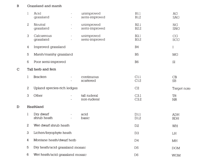
Phase1 codes
After you have finished digitising all the regions that overlap each other will be removed. The ids remaining will be the lowest id number of the two in the overlapping areas. So the polygons that you draw first will take priority. Start with small areas and draw the large areas last.
Run this in the console
digitise(shp=“phase1.shp”)
Go full screen by clicking on the second icon (show in new window) along the top of the map.

Plan your digitising strategy before starting. Switch to Esri imagery (satellite) and try zooming in. There is a limit to the resolution, so you can’t digitise more precisely than this. Think about the “minimum mappable area.” In any mosaic habitat there will be small patches of alternative habitat. How small do they have to be before you ignore them?
Digitise slowly and carefully. Start with the smaller areas and work up. Remember that any overlaps will be removed sequentially with the first polygon that is digitised taking preference over the next.
Click done when you have finished.
On completing the digitising you will find the shapefile(s) have been added into your folder. You can see them in the files tab in the bottom right.
4.2 Read the file into R
The file is called “phase1.shp.” It can be read into R memory with a single line. Note that st_read brings the data into R’s memory from the file. The data is assigned to an object that is named phase1. The object name and the file name do not have to be the same.
phase1<-st_read("phase1.shp")To ensure that the coordinates are in the British National grid CRS we can run a transform. The EPSG code for the British national grid is 27700. This line transforms coordinates in latitude and longitude (unprojected) into British national grid (projected). Global data sets will typically be unprojected. Changing the CRS is a common step in GIS and is quick and easy. Even if the data are in British national grid there is no harm in running the line in order to ensure consistency. If you run any measurements or calculate buffers for unprojected data the results will be in degrees, which are clearly not interpretable. Results calculated on projected data will be in meters.
phase1<-st_transform(phase1,27700)A geoprocessing function now needs to be run in R to cut out all the overlapping areas through differencing.
phase1<-st_difference(phase1)There are several common geoprocessing operations which can be shown in the form of Venn diagrams. A useful reference is Robin Lovelace’s online book, found here
https://geocompr.robinlovelace.net/geometric-operations.html

Examples of geoprocessing operations
You can look at the result using mapview.
mapview(phase1, zcol="id", burst=TRUE)4.3 Adding attributes
Now comes a potentially rather tricky, but very important part. In order to link the ids with any data you might have collected in the field you will need a file with this field data. You can make one in Excel on your PC, save it as a csv and upload it to the server.
This approach will work for any data you might collect in the field that you want to link to digitised objects. You just need to make sure that you know the id of the objects with spatial coordinates (which may be points, lines or poygons) and make sure that the data you have collected also has an id column that matches these.
So, if your file is called p1.csv it would look like this after uploading and reading into R. The aqm::dt function is used to form an Excel type table in the markdown document you are looking at. The actual table would of course be formed in excel and would look exactly the same. Save it as a csv then upload it ot the server.
p1<-read.csv("p1.csv")
aqm::dt(p1)
Notice that there is a single column that matches the id column in the digitised data and a second column that represents the phase1 mapping code from the handbook. The link between the codes themselves and the habitat types can also be turned into another simple table and uploaded to the server as “handbook.csv.”
Again you should form your own table in Excel, save as a csv and upload. The codes must be identical to those in the file you will merge it with for this to work.
handbook<-read.csv("handbook.csv")
aqm::dt(handbook)
Now, to put all this together the files are merged together. The common column headers result in the additional columns being added. BE VERY CAREFUL NOT TO HAVE MORE THAN ONE COLUMN NAME THAT MATCHES!.
If you try to merge two tables with more than one matching column the results will not be interpretable.
phase1<-merge(phase1,p1)
phase1<-merge(phase1,handbook)
aqm::dt(phase1)
Now when we look at the result you can see a map with habitat names showing.
Finding a good colour scheme is the tricky part. R will understand simple names for colours. So we could make them into red and green.
phase1<-st_difference(phase1)
mapview(phase1, zcol="habitat", col.regions=(c("red", "green")))
4.4 Finding hex codes for colours
This may not be so good for the colour blind. Finding perfect colours can be difficult, but using colour wheels and other similar tools can help to find more subtle combinations.
https://www.color-hex.com/color-wheel/
Replace the names for the hex codes taken from the colour wheel. This can be a time consuming exercise if the map is complex with many habitats, but it will eventually produce an acceptable result. Don’t spend too much time on this for the current exercise.
mapview(phase1, zcol="habitat", burst=TRUE,col.regions=(c( "#8d6435", "#718d35")))4.5 A simple analysis using buffering
What if you want to find all the habitat within a certain distance from the paths? You might first want to digitise the paths.
Run this in the console
digitise(shp="paths.shp)
Choose the lines button for digitising and draw some paths.
paths<-st_read("paths.shp")To make sure you are working in OS grid coordinates again.
paths<-st_transform(paths,27700)mapview(paths)4.5.1 Buffering
A very common operation in any GIS involves buffering around one object to enlarge it by the buffer distance. When the buffer is overlain on another spatial layer and the difference taken the result is the areas of the layer that fall outside the buffer. So to just look at the area of the field that is 50m from the paths, buffer and difference.
paths_buffer<-st_buffer(st_union(paths), 50)The buffer looks like this.
plot(paths_buffer)
phase1_core<-st_difference(phase1,paths_buffer)We can then look at this core area.
phase1_core$area<-st_area(phase1_core)
mapview(phase1_core, zcol="habitat", burst=TRUE,col.regions=(c( "#8d6435", "#718d35"))) + mapview(paths)
This table shows the total areas.
phase1_core %>% group_by(habitat) %>%
  summarise(area=sum(area)) %>%
  st_drop_geometry() %>% aqm::dt()
You could find all the habitat within the buffer by using the st_intersection function.
phase1_edge<-st_intersection(phase1,paths_buffer)
phase1_edge$area<-st_area(phase1_edge)
mapview(phase1_edge, zcol="habitat", burst=TRUE,col.regions=(c( "#8d6435", "#718d35"))) + mapview(paths)
4.6 Finding distances between geometries
To find the distances from each of the polygons to the nearest path.
phase1$path_distance<-st_distance(phase1,st_union(paths))
mapview(phase1, zcol="habitat",col.regions=(c( "#8d6435", "#718d35")))
4.7 Conclusion
At this stage you would certainly not be expected to understand why the R code produces the results shown! There is a lot going on. However the exercise shows that with experience it can be quite easy to use R as a replacement for desktop GIS. Most GIS operations in R usually involve predigitised data taken from other sources, as drawing maps from scratch is much less common now that so much spatial information has been captured online. However there are always times when you do need to capture data you collect in the field and show the data as a map.