Chapter 23 More on distances in GIS
23.1 Introduction
This class is not essential for the assignment, but will explain how the minumum distance to the nearest tree was added to the data frame. It shows some common GIS concepts in action using R including changing from raster to vector format and sampling points within polygons.
## Load libraries for spatial work.
library(tidyverse)
library(aqm)
library(giscourse)
library(sf)
library(mapview)
library(raster)
library(leaflet.extras)
library(RColorBrewer)
pal1<-terrain.colors(100)
pal2<-gray(0:100 / 100)
First load up the data from Arne.
data("arne_pines")
d<-arne_pines
## Remember how to produce a spatial object from this data frame
# Make it spatial
d<-st_as_sf(arne_pines,coords = c("lon","lat"),crs=4326)
# Reproject to national grid
d<-st_transform(d,27700)
Now load up the lidar data. We’ll crop and mask the dtm and the dsm to the study area.
data(arne_lidar)
# Just to check. Will reset old format CRS
d<-st_intersection(d,study_area)
study_area<- st_transform(study_area, 27700)
dtm<-crop(dtm, study_area)
dtm<-mask(dtm, study_area)
dsm<-crop(dsm, study_area)
dsm<-mask(dsm, study_area)
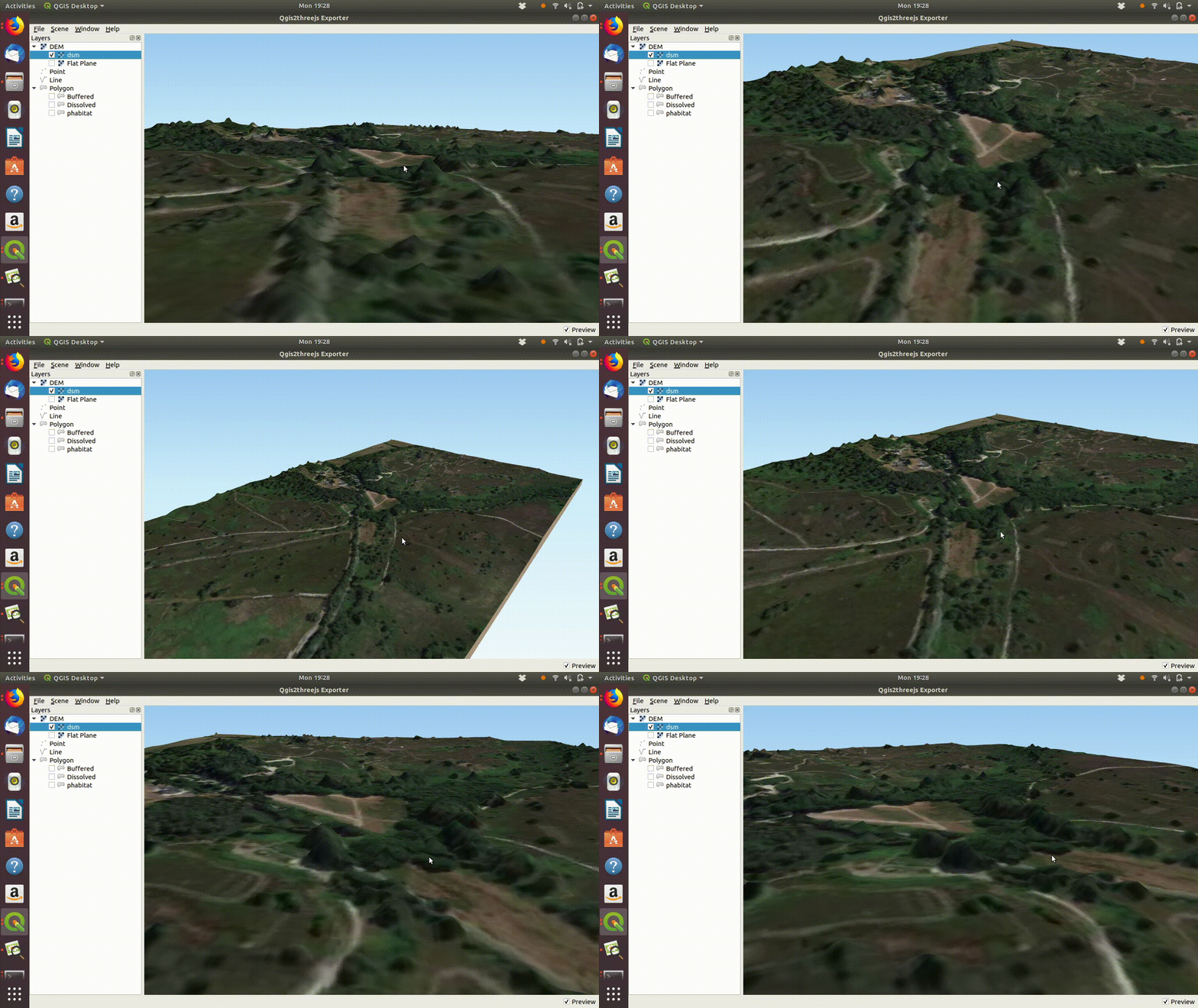
The arne DSM viewed in QGIS.

Arne digital surface model viewed in QGIS
Now to produce a canopy height model we simply subtract the dtm from the dsm
chm<-dsm-dtm
plot(chm)
Notice how this shows up the positions of the taller trees.
23.2 Vectorising the trees
In order to produce a vector layer for the outlines of the trees I used a few tricks in R. Its worth noting that there was no bespoke operation in either QGIS nor in Arc to achieve this result easily.
chm[chm<2]<-NA ## Set below 2m as blanks (NA)
chm[chm>=2]<-1 ## Set above 2m to a single value
trees<-rasterToPolygons(chm, dissolve=TRUE) # Turn to vector
trees<-st_as_sf(trees)
trees<-st_cast(trees$geometry,"POLYGON") # Make each polygon distinct
trees<-st_transform(trees,27700)
Notice that the procedure does pick out most of the individual trees on the heathland, including some that have been removed since the lidar was obtained. This can be seen by comparing the results to the satelite image.
mp<-mapview(trees)
mp@map %>% addFullscreenControl()
It is not perfect, however the laternative option of digitising each tree visually would be a very time consuming task.
23.3 Finding the distances to the trees
If we ask R for the distances between the trees and the quadrats (the object called d) we will get a large matrix of results containing the distance between each one of the quadrats and every single identified tree.
distances<-st_distance(d,trees)
dim(distances)
So if we want the distance to the nearest tree we need to run down the rows and find the minimum.
d$min_dist<-apply(distances,1,min)This does the job. A new column has been added to the object containing the shortest distance to a tree.
As the distance matrix contains all the measured distance it is possible to design bespoke functions using it to find other quantities. For example, if we wanted to know how many “trees” are within 50m of each quadrat we could use this.
# The function uses a rule (<50)
# And then sums the number of true results
count_trees<-function(x)sum(x<50)
d$n50<-apply(distances,1,count_trees)
23.4 Spatial sampling
It is clear that the students did not place the quadrats randomly over the whole potential study area. There are many reasons for this, some involved logistics and others the decisions made by the students.
What would a representative spatial sample of the area look like?
One possibility is to place the same number of quadrats completely at random within the area. This can be simulated easily in R.
random<-st_sf(name="random", geom=st_sample(study_area, 184))
distances<-st_distance(random,trees)
random$min_dist<-apply(distances,1,min)
The results are shown in the mapview produced after the next couple of code chunks. One rather surprising element of a truly random spatial sample is that to the eye it appears to be clustered. We can use R to obtain a set of points placed regularly within the area for comparison.
regular<-st_sf(name="regular", geom=st_sample(study_area, 184, type="regular"))
distances<-st_distance(regular,trees)
regular$min_dist<-apply(distances,1,min)
23.5 Mapping the results
mapview(d,col.region="orange") +
mapview(regular,col.region="darkblue") +
  mapview(random,col.region="darkred") +
  mapview(trees, col.region="darkgreen") ->map
map %>% extras()
23.6 Exercise
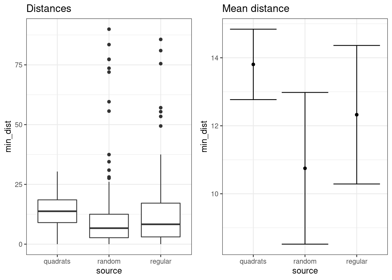
Analyse the distances from the trees from the three sources.
We can turn the results in each object into a single data frame for this exrcise.
d1<-data.frame(source="quadrats",min_dist=d$min_dist)
d2<-data.frame(source="random",min_dist=random$min_dist)
d3<-data.frame(source="regular",min_dist=regular$min_dist)
df<-rbind(d1,d2, d3)
# Hint
g0<-ggplot(df,aes(x=source,y=min_dist))
f1<-g0+geom_boxplot() +labs(title="Distances")
f2<-ci(g0) +labs(title="Mean distance")
multiplot(f1,f2,cols=2)
Figure 23.1: Notice that the quadrat data do not include some of the areas that are very distant from any trees