Chapter 22 Arne pine density: Spatial data part 1
library(tidyverse)
library(aqm)
library(giscourse)
library(sf)
library(mapview)
library(raster)
library(leaflet.extras)
library(RColorBrewer)
pal1<-terrain.colors(100)
pal2<-gray(0:100 / 100)
22.1 Introduction
In this session you wil practice using some of the GIS capabilities of R in the context of the data collected at Arne. If you have already analysed the pine growth data and the pine density data with respect to the derived variables there is not too much to add in order to complete the assignment. However the way the variables that might be related to the pine densities was actually obtained may still be rather mysterious. This class will show you how you can work with lidar derived digital elevation rasters (DEMs and DTMs)
22.1.1 Obtaining Lidar data
The repository for openly available lidar data online has changed several times in the last few years. The most comprehensive source is now held by DEFRA.
https://environment.data.gov.uk/DefraDataDownload/?Mode=survey
Downloading the data is fairly straightforward, but is still something of a hassle for use in class.The DEFRA interface can produce a large number of files for a single site. You should be aware that this data is available and can be imported into R if you are working at a specific site for your own project, but for the purposes of this unit we will use data that is already loaded. This data is a little out of date, but corresponds to the situation when the field data was collected.

22.1.2 Arne pine density measurements
The pine density data was obtained by students through the use of circular quadrats. The quadrats were georeferenced by matching the ids to waypoints from a GPS. Pine densities were calculated by dividing the number of pines found in the circular areas by the area of the circles.
data("arne_pines")
d<-arne_pines
str(d)
The actual areas varied between years as a result of the students using different lengths of rope to measure out the circles. So use the densities, not the raw counts. Notice that these data simply form a data frame. They could be loaded into R from Excel as a CSV.
22.1.3 Pine densities in heath and restauration area.
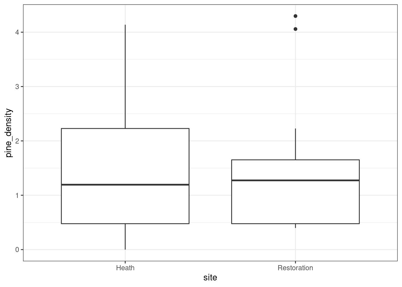
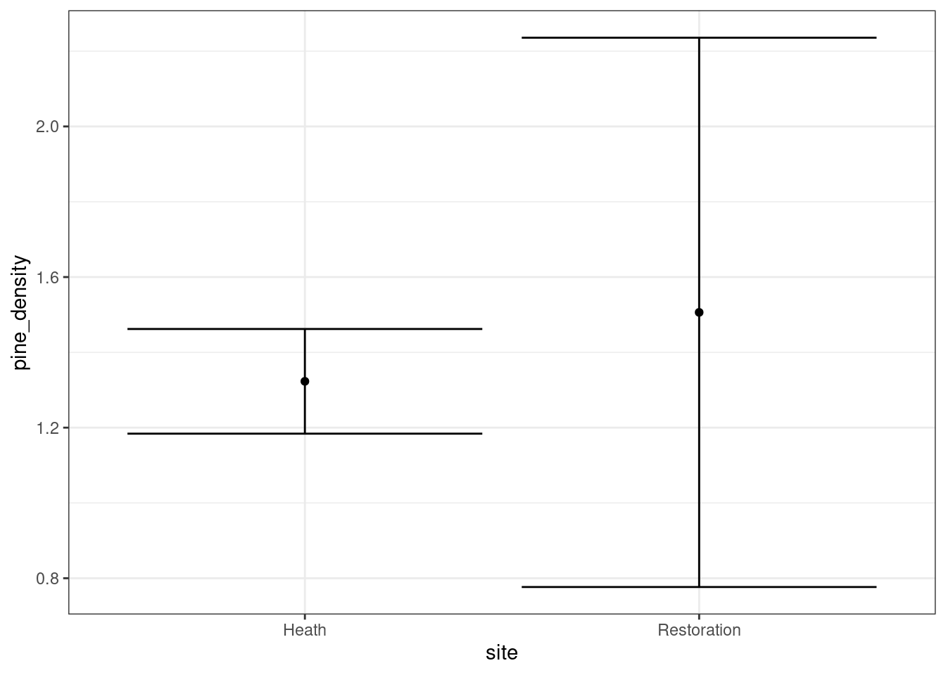
The data is not very representative of the two areas due to very limited sampling. However you can apply a simple t-test based approach to look at any differences between densities in the two areas. Strong caveats apply.
If you are concerned about the work to include in the assignment please do note that this whole section is an optional extra. It is not strictly needed to complete the assignment as set. However it is always useful to practice applying the methods shown on the unit in different contexts in order to become more comfortable with them.
g0<- ggplot(d,aes(x=site,y=pine_density))
g0+geom_boxplot()
aqm::ci(g0)
What would a t test show?
22.1.4 Making a spatial object
In order to turn them into a spatial object we need to tell R something about them.
We know that the x coordinates are the longitude (lon) and the y coordinates are the latitude (lat). These are not projected so the coordinate reference system (CRS) is 4326. If the points had been collected in OS national grid form then the CRS would be 27700. We can transform to National Grid easily after loading data in aLatitude and Longitude CRS.
d<-st_as_sf(arne_pines,coords = c("lon","lat"),crs=4326)
d<-st_transform(d,27700)
Now we can map the positions. If you want a full screen control this is added using the leaflet.extras package. By making year the zcol and “bursting” the data the map will show a layer for each year and a legend if legend is true, or without in this case.
mapviewOptions(homebutton = FALSE)
map<-mapview(d, zcol="Year", burst=TRUE, legend=FALSE)
map@map %>% leaflet.extras::addFullscreenControl()
Adding a minimap also uses the leaflet.extras package. The lower the negative value for the zoomLevelOffset the greater the difference in scale between the two maps. You can also select different base maps. This can be useful for showing the position of a study site.
map@map %>% addFullscreenControl() %>%
  addMiniMap(position = "bottomleft",tiles="OpenStreetMap",zoomLevelOffset = -6, toggleDisplay=TRUE) %>%
  addScaleBar(pos="bottomright")
22.1.5 Loading the lidar data
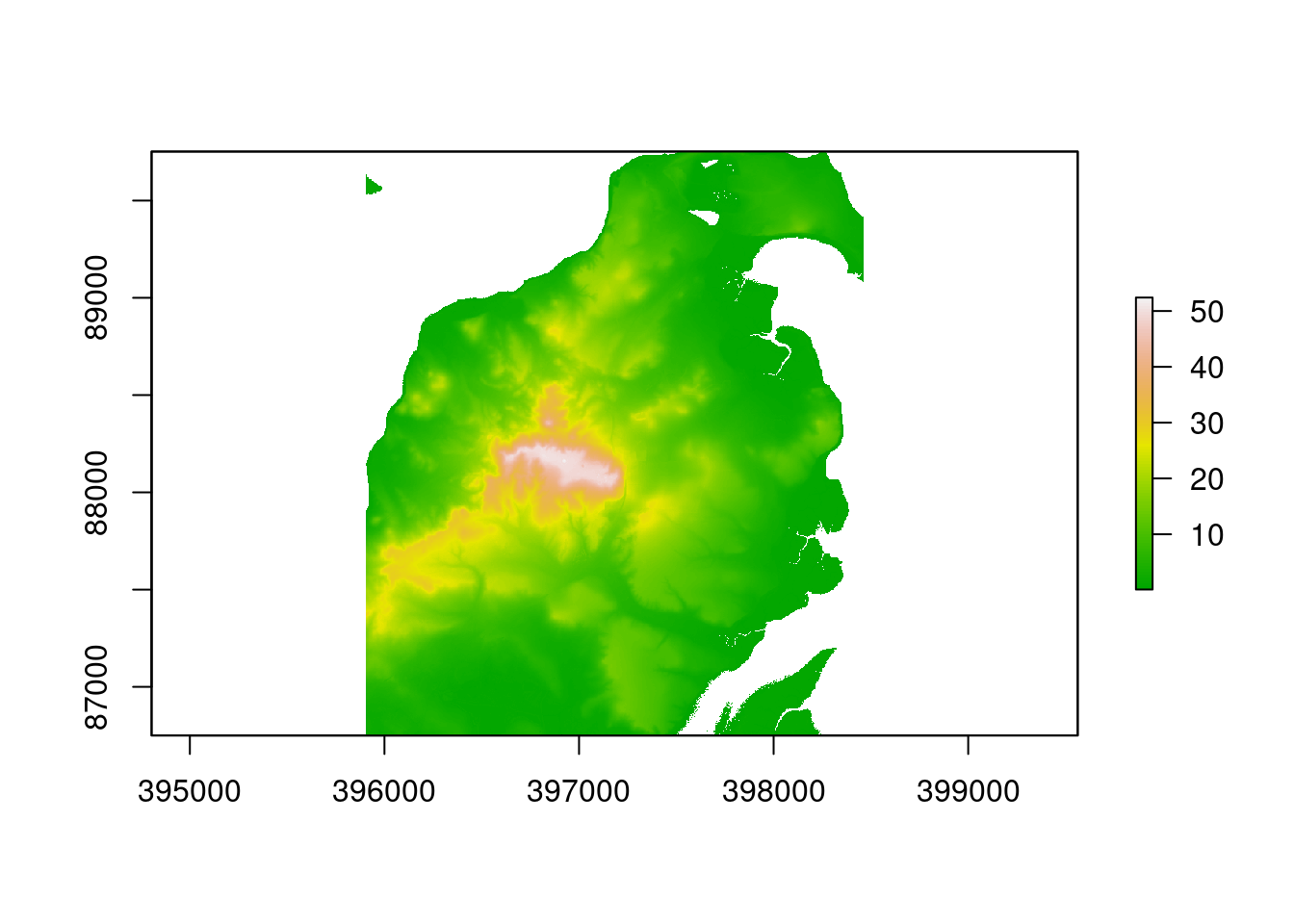
The following line loads the saved Lidar derived 2m DTM and DSM layers for the Arne area together with a polygon representing the study site.
data(arne_lidar)A quick plot of the dtm shows the layer.
plot(dtm, col=pal1)
22.1.6 Exercise
Use the code from the previous class to produce a shaded hill layer for Arne and display this as a map.
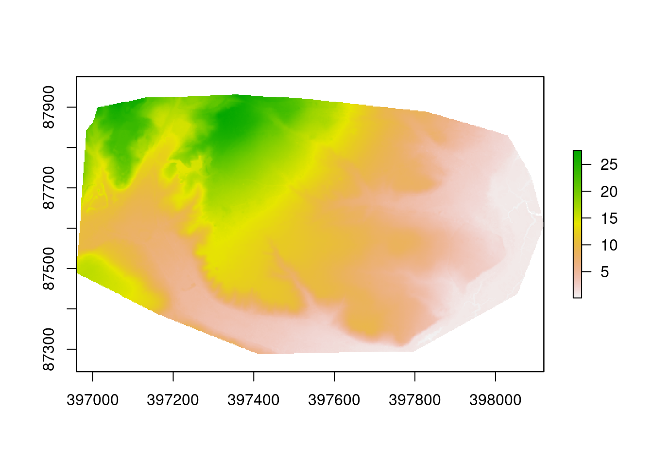
22.1.7 Cropping and masking to the study site
The code also loaded a polygon representing the heathland study area. A sing
dtms<-crop(dtm, study_area)
dtms<-mask(dtms, study_area)
plot(dtms)
22.1.8 Exercise
1.Crop and mask the DSM
Derive a canopy height model for the study are and plot it. A canopy height model is the difference between the DSM and DTM. It can be found by a simple map algebra operation.
Play around with the maps you have. Try deriving slope aspect and hillshades and plotting them out using code from the last class.
22.1.9 Using only the data from the study site
To remove any quadrats that fall outside the study are we can use a geoprocessing operation to find the intersect.
d<-st_intersection(d,study_area)To find the elevation at any of the points we use the extract function in the raster package.
d$dtm<-raster::extract(dtms, d)Now if you look at the object you will see that the relevant values have been added. This process can be repeated for any raster layer derived from the two layers.
22.1.10 Extracting additional data from the raster layers
The giscourse package contains a couple of functions to use the SAGA algorithms ta_hydrology and ta_lighting to extract a topographic wetness index (twi) and daily direct beam insolation from the digital terrain model.
If we bundle laters together as a raster brick the extract function only needs to be run once to extract all the values and assign them to the spatial object.
insol<-giscourse::insol(dtms)
names(insol)<-"insol"
twi<-giscourse::twi(dtms)
names(twi)<-"twi"
slope<-terrain(dtms,"slope")
aspect<-terrain(dtms,"aspect")
lyrs<-raster::brick(insol,twi,slope,aspect)
d<-cbind(d,raster::extract(lyrs, d))str(d)22.1.11 Finding distance from paths
The open street map layer that you can see as a basemap can also be downloaded as a vector layer. The process of doing this is a little complex, so I have done this for you and placed the data in the aqm package.
data(arne_paths)
paths<-st_intersection(paths,study_area)
mapview(paths)
Now if we want to add the distance from the path to each quadrat it is easy.
d$path_dist<-st_distance(d,paths)