Section 17 Appendix: Writing SQL: Some tips and tricks
require(RPostgreSQL)
require(rpostgis)
require(sf)
require(tmap)
require(mapview)
conn <- dbConnect("PostgreSQL", host = "postgis",
  dbname = "gis_course" ,user = "gis_course", password = "gis_course123")
17.1 General advice
The gis_course user connection is limited to 30 seconds. If a query is written that over runs this limit it will time out with no results. This can occur when you are new to postgis.
- Find out what you are looking for. You can’t write a correct query if you don’t know table and field names. See 17.2, 17.3, 17.5.
- Know the size of the table you are working with. Postgis is designed for big data. However very big data might not all load into memory or may not display as a map. 17.4 helps.
- Test queries carefully setting limits at first if the table is large 17.6
- Use the right sort of call to the data base from R 17.8
- Learn to use sprintf in R to help build complex queries from sub queries 17.11
- Apparently slow queries may actually be slow because the results take time to render. Learn to use st_simplify with complex geometries 17.12.
17.2 Find table names in R
It is a good idea to pipe this into a searchable table when writing in markdown. Write a few letters in the search tab to find your table.
dbListTables(conn) %>% data.frame() %>% DT::datatable()17.3 Find field names in R
dbListFields(conn,"sssi") %>% data.frame() %>% DT::datatable()17.4 Count the number of records in a table
You can choose any named field to get a count.
query<-"select count(gid) from sssi"
dbGetQuery(conn,query)
#>   count
#> 1  9510
17.5 Find all possible values of a categorical field
query<- "select distinct sssi_name from sssi"
dbGetQuery(conn,query)  %>% as.data.frame() %>% DT::datatable()
17.6 Set limits to queries when testing them
The safe way to design queries is to set a limit when writing them. This applies to R or QGIS db manager. A useful trick is to include order by random if you don’t want to get just the first 10 values.
query<- "select * from sssi order by random() limit 10"
sssi<-st_read(conn,query=query)
This can be turned into a little function for safe testing a query.
safe_test<-function(sql=sql,n=10){
  query<-sprintf("%s order by random() limit %s",sql,n)
  st_read(conn,query=query) %>% st_set_geometry(NULL) %>% DT::datatable()
}
query<- "select * from sssi"
safe_test(query)
17.7 Add a unique identifier
Tables in postgis might not have a unique ID column for many reasons. You don’t need one in R. However you do in QGIS in order to load the table.
Just add ROW_NUMBER () OVER () id to the query. ** Note this assumes that id does not exist as a name. If it does, change the alias**
Demo in R, but for use in QGIS db manager.
query<-"select ROW_NUMBER () OVER () id , sssi_name,geom from sssi"
safe_test(query)safe_test("select * from nat_earth_uk",100)
#> type is 13717.8 DbSendQuery, DbGetQuery and st_read
There are three functions for working with queries in R.
17.8.1 DbSendQuery
DBSendQuery does not return data, but sets things up in the data base. For example this query sets up a table for Dorset, Poole and Bournemouth that may be useful when subsetting.
dbSendQuery(conn, "drop table if exists dorset;")
#> <PostgreSQLResult>
dbSendQuery(conn, "create table dorset as
           select ROW_NUMBER () OVER () id,
            ctyua16nm nm, geom from counties
            where ctyua16nm in ('Dorset','Poole','Bournemouth')")
#> <PostgreSQLResult>
17.8.2 st_read
To get the results with the geometries for mapping use st_read. By default this reads a whole table. If you want a query you must state query= query.
st_read(conn,"dorset") %>% qtm()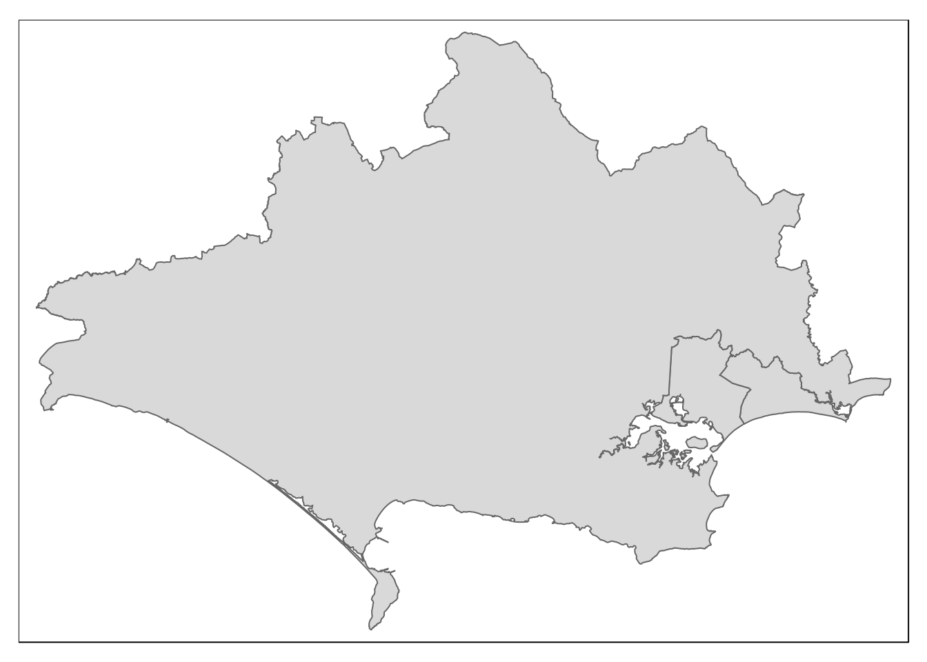
## Same with a query
#st_read(conn,query= "select * from dorset") %>% qtm()
17.9 dbGetQuery
The st_read function is designed for spatial data. It won’t work correctly if there is no geometry column. Use DbGetQuery in this case. For example to find the 10 largest SSSIs without returning their geometry.
dbGetQuery(conn,"select sssi_name,
round(st_area(geom)/10000) areaha from
sssi order by areaha desc limit 10")
#>                   sssi_name areaha
#> 1                  The Wash  62038
#> 2            Humber Estuary  36979
#> 3            The New Forest  28596
#> 4             Morecambe Bay  25165
#> 5          North York Moors  23324
#> 6             Bowland Fells  16008
#> 7                 Dark Peak  15464
#> 8            Upper Teesdale  14365
#> 9  Moorhouse and Cross Fell  13817
#> 10           North Dartmoor  13559
17.10 Checking coordinate reference system
Piping a single geometry to st_crs is one quick way of finding out the crs used by postgis when working in R.
st_read(conn, query ="select geometry from gbif limit 1") %>% st_crs()
#> Coordinate Reference System:
#>   EPSG: 4326
#>   proj4string: "+proj=longlat +datum=WGS84 +no_defs"
st_read(conn, query ="select geom from counties limit 1") %>% st_crs()
#> Coordinate Reference System:
#>   EPSG: 27700
#>   proj4string: "+proj=tmerc +lat_0=49 +lon_0=-2 +k=0.9996012717 +x_0=400000 +y_0=-100000 +ellps=airy +towgs84=446.448,-125.157,542.06,0.15,0.247,0.842,-20.489 +units=m +no_defs"
st_read(conn, query ="select geometry from waterways limit 1") %>% st_crs()
#> Coordinate Reference System:
#>   EPSG: 27700
#>   proj4string: "+proj=tmerc +lat_0=49 +lon_0=-2 +k=0.9996012717 +x_0=400000 +y_0=-100000 +ellps=airy +towgs84=446.448,-125.157,542.06,0.15,0.247,0.842,-20.489 +units=m +no_defs"
17.11 Using sprintf
The sprintf function in R can help when building large queries. This function acts like paste, but is easier to use in many respects. The logic is that the %s place markers in a sprintf query gets filled in with the values of the variables placed at the end.
17.11.1 Saving typing field names
Here’s one useful trick with sprintf. The * operator in sql selects all the fields. However it is not good practice to pull in lots of information we don’t want with a query. Annoyingly in SQL there is no way of dropping just the geometry field if we don’t want it. We can get all the fields on a table with dbListFields.
fields<-unlist(dbListFields(conn,"nat_earth_uk"))
fields
#>  [1] "featurecla" "scalerank"  "adm1_code"  "diss_me"    "iso_3166_2"
#>  [6] "wikipedia"  "iso_a2"     "adm0_sr"    "name"       "name_alt"
#> [11] "name_local" "type"       "type_en"    "code_local" "code_hasc"
#> [16] "note"       "hasc_maybe" "region"     "region_cod" "provnum_ne"
#> [21] "gadm_level" "check_me"   "datarank"   "abbrev"     "postal"
#> [26] "area_sqkm"  "sameascity" "labelrank"  "name_len"   "mapcolor9"
#> [31] "mapcolor13" "fips"       "fips_alt"   "woe_id"     "woe_label"
#> [36] "woe_name"   "latitude"   "longitude"  "sov_a3"     "adm0_a3"
#> [41] "adm0_label" "admin"      "geonunit"   "gu_a3"      "gn_id"
#> [46] "gn_name"    "gns_id"     "gns_name"   "gn_level"   "gn_region"
#> [51] "gn_a1_code" "region_sub" "sub_code"   "gns_level"  "gns_lang"
#> [56] "gns_adm1"   "gns_region" "min_label"  "max_label"  "min_zoom"
#> [61] "wikidataid" "name_ar"    "name_bn"    "name_de"    "name_en"
#> [66] "name_es"    "name_fr"    "name_el"    "name_hi"    "name_hu"
#> [71] "name_id"    "name_it"    "name_ja"    "name_ko"    "name_nl"
#> [76] "name_pl"    "name_pt"    "name_ru"    "name_sv"    "name_tr"
#> [81] "name_vi"    "name_zh"    "ne_id"      "geometry"
Now we can use sprintf to choose which of the fields from 1 to 84 we want to include without typing them out.
query<-sprintf("select %s from nat_earth_uk",paste(fields[c(3,9,84)],collapse=","))The query now reads
select adm1_code,name,geometry from nat_earth_uk
st_read(conn,query=query) %>% mapview()17.11.2 Using sprintf to join sub queries
This is a very handy trick which avoids typing complex queries in one go. It is especially useful for spatial intersects and geoprocessing involving two or more tables.
focal_area<-"select geom from counties
            where ctyua16nm in
('Hampshire','Wiltshire')"

st_read(conn,query=focal_area) %>% qtm()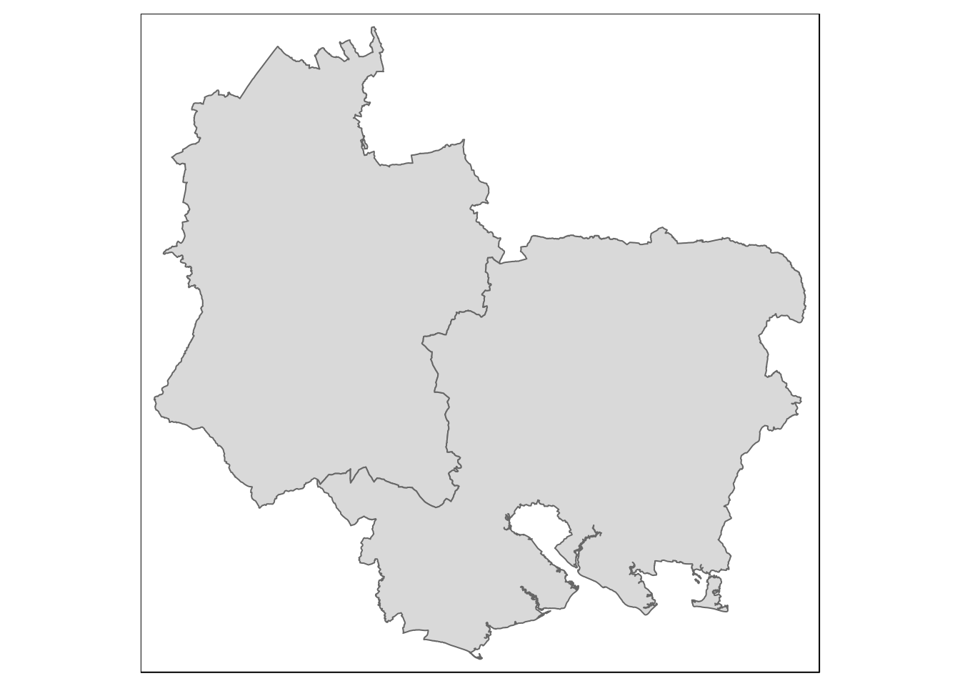
query<-sprintf("select st_simplify(s.geom, 100)
  from sssi s, (%s) l where
  st_intersects(s.geom, l.geom) ",focal_area)
The query now reads
select st_simplify(s.geom, 100) from sssi s, (select geom from counties where ctyua16nm in (‘Hampshire’,‘Wiltshire’)) l where st_intersects(s.geom, l.geom)
st_read(conn,query=query) %>% qtm()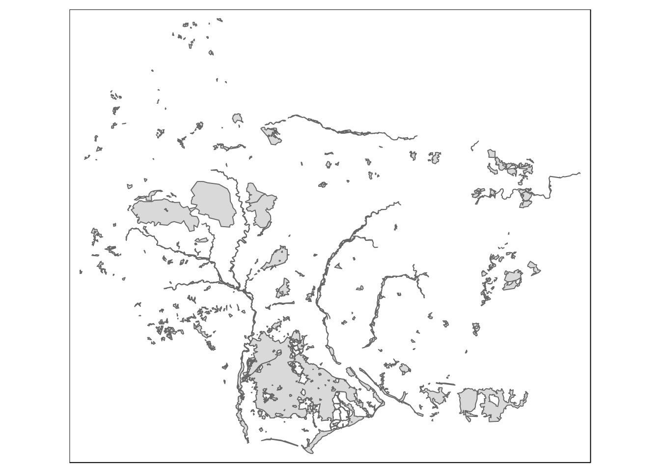
17.12 Using st_simplify
Complex geoemtries are slow to render and can freeze up the system even though the query does not take long to run. Geometries should be simplified to the appropriate scale for map making. For example if just want to draw the county boundaries of England and Wales we can simplify radically.
st_read(conn, query="select ctyua16nm,st_simplify(geom,1000) from counties") %>% qtm()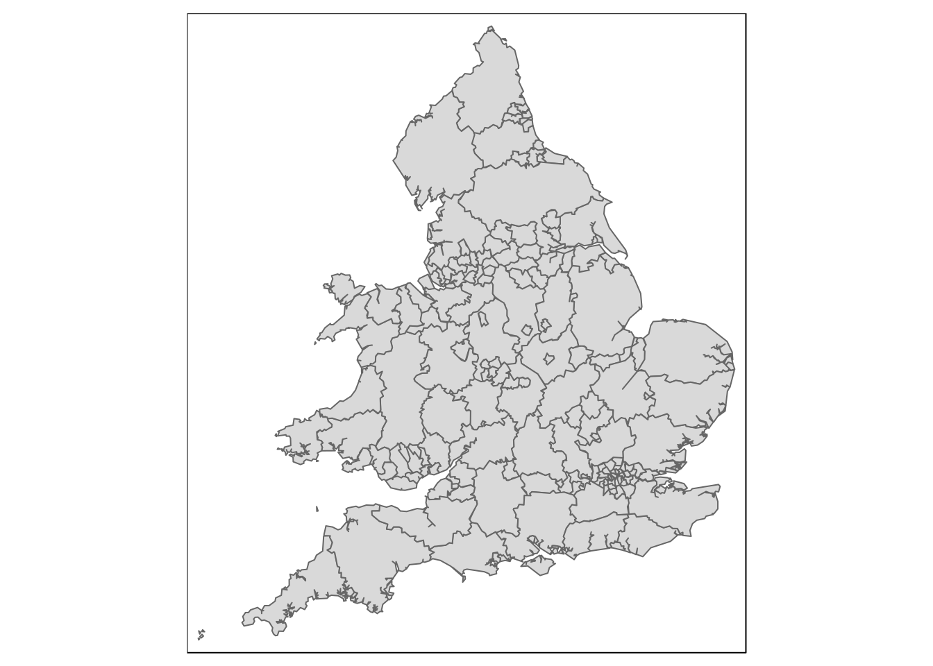
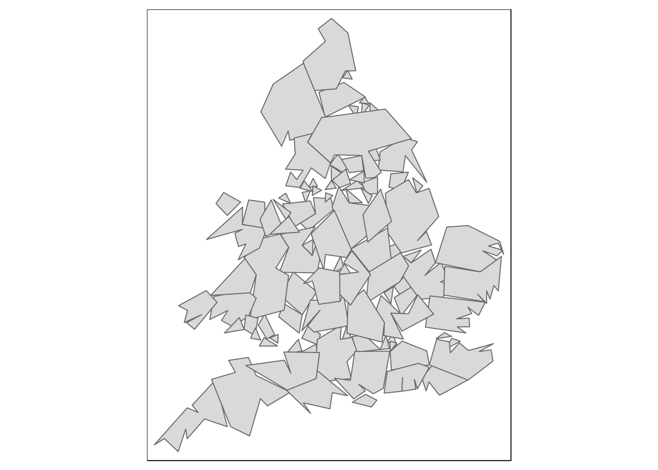
Notice that the process can be taken too far.
st_read(conn, query="select st_simplify(geom,10000) from counties") %>% qtm()