Section 10 Terrain analysis

10.1 Concepts

Terrain analysis involves the analysis of topographic features (geomorphology). The operations required typically take raster layers as input,although three dimensional point cloud data can also be used directly for some analyses. The input to most forms of terrain analyses are digital elevation models (DEMs). These can take various forms.Traditionally they were produced through interpolation between contours from a traditional map. DEM’s are now mainly derived from remote sensing involving some form of radar based sensor. For example

- SRTM (Shuttle Radar Topography mission): Global extent 90m resolution
- Lidar (Light detection and ranging): Local extent, varying resolution

Raw lidar data consists of a point cloud of returns with some additional information regarding the intensity of the return. The point cloud has two key reference points. The first return represents the top of vegetation or buildings and the last return should typically be the ground

Lidar point clouds can be processed to form digital terrain models (DTMs) by taking the last returns and using smoothing and interpolation. Digital surface models use the first return. This processing can be achieved using a range of different software. For example QGIS can be linked to LASTools to process point clouds directly.

Terrain analysis uses algorithms to calculate a potentially large number of different derived layers from the digital terrsin models and the digital surface models. These typically include slope, aspect, hillshading and elements such as direct beam insolation and topographic wetness index.

There are many uses for terrain analysis. Hydrologists can use it to delimit watersheds and analyse flows. The layers derived from terrain analysis can be queried to produce information at points, along lines or within polygons. We can also carry out raster alegebra operations on the layers.

https://rpubs.com/dgolicher/lidar

To see some point clouds open http://plas.io/ and load the lidar data from the course web site (link to be added)

Figure 10.1 shows the results.

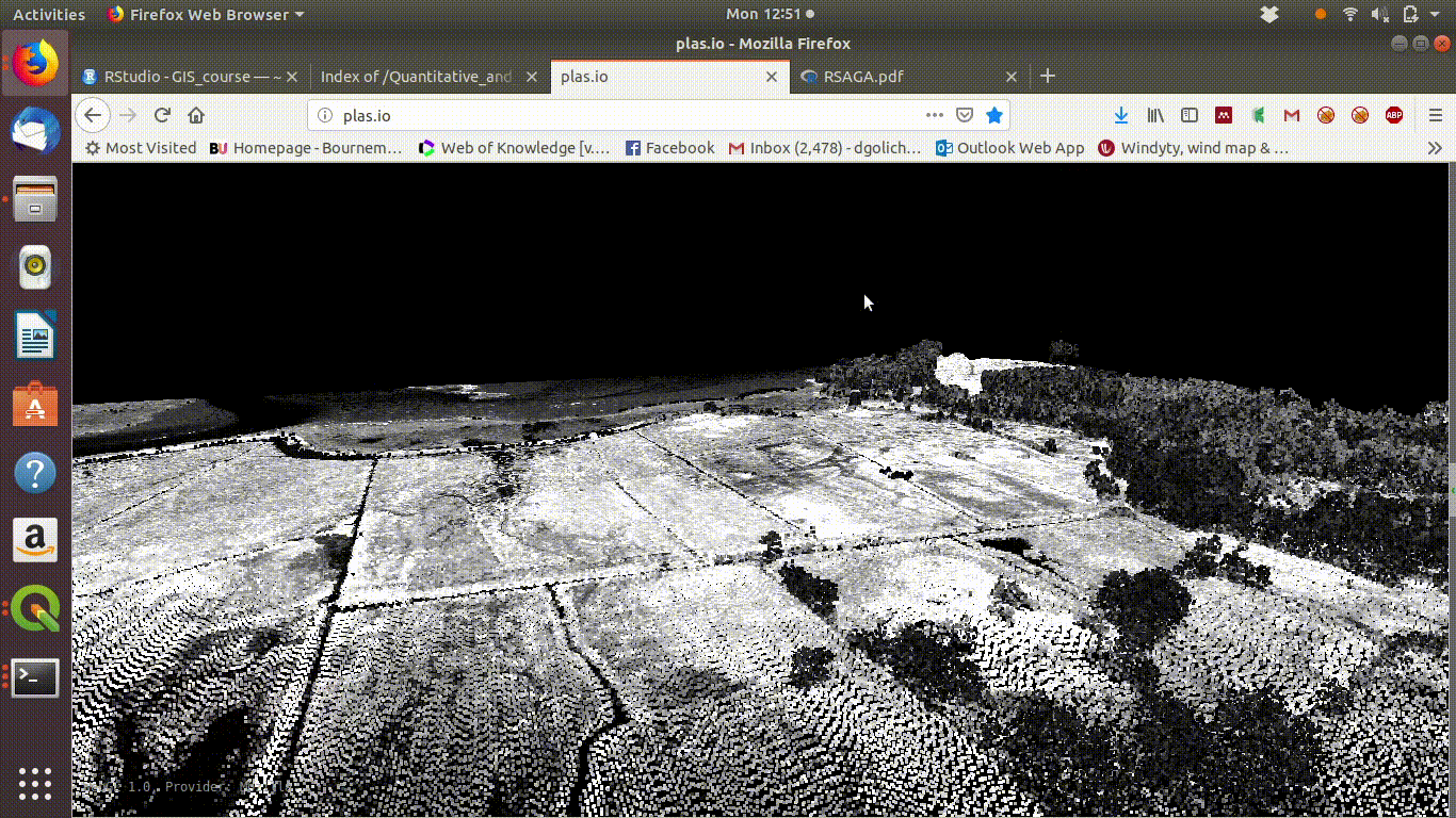
Figure 10.1: Visualising the Lidar point cloud for the Arne site using plas.io

Here are some point clouds of Arne. Download them locally then open with plas.io.

http://r.bournemouth.ac.uk:82/Quantitative_and_Spatial_Analysis/Week_2/point_clouds/

Processing the point cloud (not conducted in this class) leads to the production of Digital surface model (DSM) and th Digital terrain model (DTM)

The digital surface model is obtained by smoothing the first returns in order to produce values for a two dimensional (x and y) raster grid placed on the point cloud. The third dimension is now the value of the pixel. The resolution can be chosen when producing the model. it can’t be finer than the typical gaps between points, but it can be coarser.

The digital terrain model is obtained by smoothing the last returns with some interpolation techniques included to smooth around hard surfaces in order to produce values that should correspond to the ground surface. In cities and towns this will be more challenging than in areas with vegetation, as returns from the actual ground may be difficult.

Archeologists and geomorphologists are often interested in the visual aspect of terrain analysis. Techniques such as analytical hill shading can reveal subtle surface features that would be otherqise hidden from view. As Lidar penetrates through many types pf vegetation analysis of Lidar derived digital surface models have been used to find Mayan ruins beneath tropical forest.

In many ecological studies the main purpose behind running terrain analysis is to derive variables that can be combined with others within a quantiative analysis. For example if we place a set of quadrats down within a study area in order to look at the relationships between vegetation types and other variables we may want to know variables such as slope and aspect. Rather than try to measure this on the ground, we can easily add the values to the analysis if have derived them from a dtm and we have the coordinates of the quadrats using a gps. In many studies it is preferable to derive more informative variables than slope and aspect. For example slope and aspect combined determine how much direct beam insolation the surface recieves on a given day. This could be useful in a study of butterflies or small reptiles that may seek warm micro climates. Rather than just looking at slope, the position on a slope may be useful. There are a wide range of options that can be explored.

10.2 R

This time we will begin the practical section by looking at how to run some basic terrain analysis in R rather than QGIS. The reason for this is that some results will be passed through postgis into QGIS.

10.2.1 Required packages

Notice that we need to load rpostgis for this. The package has a useful function for reading raster data stored in a postgis data base.

library(giscourse)
require(raster)
require(mapview)
require(tmap)

mapviewOptions(basemaps =c("OpenStreetMap","Esri.WorldImagery",
                           "Esri.WorldShadedRelief", 
                           "Stamen.Terrain"))

conn <- connect()

The first step is to retrieve the habitat layer from the Arne schema in order to find the bounds of the studya area.

query1<-"select * from arne.phabitat"
arne_habitat<-st_zm(st_read(conn,query=query1))
bound<-as(arne_habitat, "Spatial")

Section 18.7 explains how lidar data was loaded onto the server. The data on the server are continuous 2m resolution digital surface model and digital terrain models for the OS grid squares around Arne and Hengistbury head. There is no coverage of other areas in this data base, although it could be added by downloading the data from the online source and running through the script in section 18.7.

The following lines clip the layers to the bounds of the sssi. Note this is clipping to the bounds, but not masking by the polygon.

dsm<- pgGetRast(conn, "dsm2m",boundary=bound)
dtm<- pgGetRast(conn, "dtm2m",boundary=bound)

dsm[dsm<0.1]<-NA
dtm[dtm<0.1]<-NA

10.2.2 Summaries of raster layers

In R raster layers are handled in a similar way to other matrices. So native R functions such as hist will work directly on the layer. So will the summary.

hist(dtm)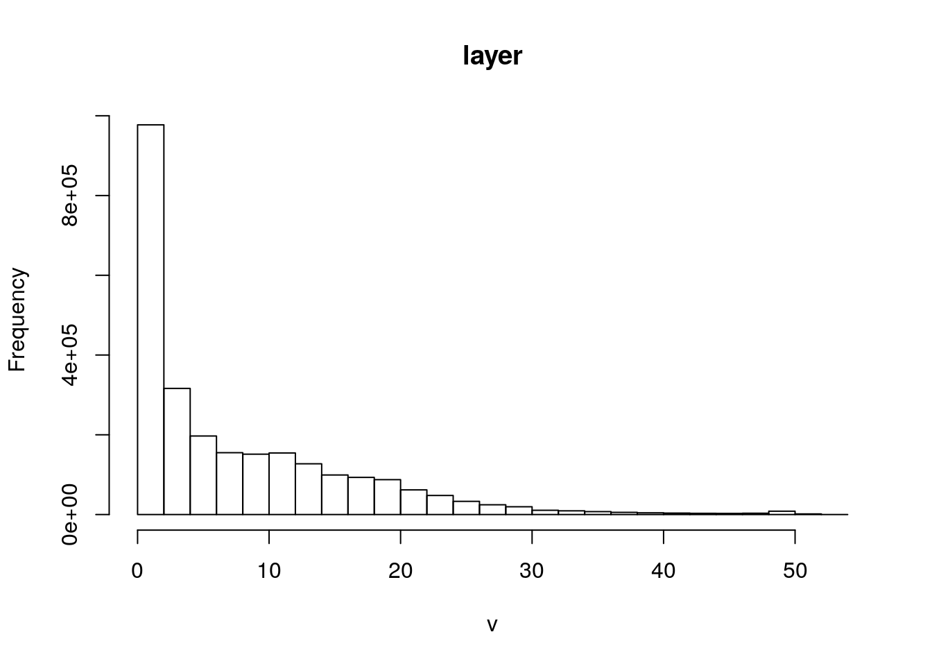

Figure 10.2: Simple histogram of the digital terrain model for Arne. Note the distribution of the elevations. Most of the site lies just a few meters above sea level with a maximum of 52m above sea lavel.

summary(dtm)
#>              layer
#> Min.         0.100
#> 1st Qu.      0.998
#> Median       4.073
#> 3rd Qu.     12.038
#> Max.        52.665
#> NA's    950690.000

10.2.3 Visualising the layers

The digital surface model and digital terrain model differ from each other markedly in areas of forest. Zoom in on the web map below and switch between layers to see the differences.

contours<-rasterToContour(dtm,nlevels=10)

require(RColorBrewer)
pal<-terrain.colors(100)

pal <- colorRampPalette(pal)

mapview(dsm,col.regions=pal, legend=FALSE) + 
mapview(dtm,col.regions=pal) + mapview(contours)

10.2.4 Deriving new terrain layers

It is extremely quick and easy to form new layers in R representing slope and aspect in R using the terrain function. Simply specify the derived layer and the units (both slope and aspect can be measured in degrees or radians)

The hillshading algorithm in R takes slope and aspect in radians as input values.

slope<-terrain(dtm, opt='slope', unit='degrees')
aspect<-terrain(dtm, opt='aspect',unit='degrees')
sloper<-terrain(dtm, opt='slope', unit='radians')
aspectr<-terrain(dtm, opt='aspect',unit='radians')
hillshade<-hillShade(sloper,aspectr,angle=5)


plot(hillshade, col = gray(0:100 / 100), legend = FALSE)
plot(dtm, col = terrain.colors(25), alpha = 0.3, legend = TRUE, add = TRUE)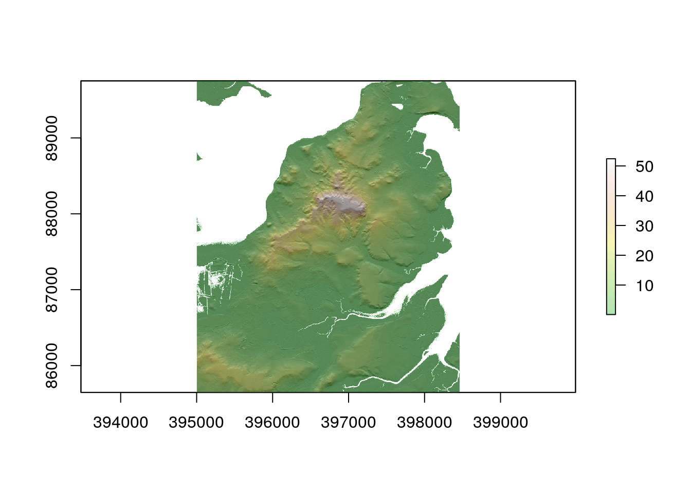

#plot(contours,add=T,col="white")

10.2.5 Saving the results and passing to QGIS through postgis

If you were running RStudio locally, i.e. not through a web based server, files produced by R could be simply saved in the QGIS project directory and added to a QGIS project as local layers.

The Rtudio version that runs on apps anywhere could possibly be used for this. However you would need to install many extra packages before it had the functionality of the server version. It cannot run saga commands and it is not linked directly to the postgis container. So to run the code as shown in this course you must use the server version.

The code below writes all the results to a subfolder of the directory in which the script is run with the path /rasters/area.

## Folder /rasters/arne must exist !

writeRaster(dsm,"rasters/arne/dsm.tif",format="GTiff", overwrite=TRUE)
writeRaster(dtm,"rasters/arne/dtm.tif",format="GTiff", overwrite=TRUE)
writeRaster(slope,"rasters/arne/slope.tif",format="GTiff", overwrite=TRUE)
writeRaster(aspect,"rasters/arne/aspect.tif",format="GTiff", overwrite=TRUE)

10.2.6 Using SAGA commands from R

SAGA (System for Automated Geoscientific Analyses) is a free and open source GIS currently maintained by a group at the university of Hamburg. http://saga-gis.sourceforge.net/en/. SAGA has some very good algorithms for terrain analysis and hydrology. However using SAGA directly would involve learning a new GUI. Providing SAGA is installed on the system it can be called from a command line. So the lines of code below use saga commands to produce a total direct beam solar insolation layer for a given day and a topographic wetness index.

See links for details and references of the specific methodology used.

http://www.saga-gis.org/saga_tool_doc/2.3.0/ta_lighting_2.html

Note that the SAGA TWI is a slight improvement on the original which works more effectively for flat valleys.

http://www.saga-gis.org/saga_tool_doc/2.3.0/ta_hydrology_15.html

Although the process looks complicated to implement all that is required is careful reading of the SAGA manual in order to choose input options to the algorithms.

## Write out the raster in saga format first.
writeRaster(dtm,"rasters/arne/saga_dtm.sgrd",format="SAGA", overwrite=TRUE)

## Run the commands (WILL ONLY WORK IF THE LIBRARIES ARE INSTALLED) 

system ("saga_cmd ta_lighting 2 -GRD_DEM 
        rasters/arne/saga_dtm.sgrd  -DAY '13/10/19' -GRD_DIRECT    rasters/arne/saga_sol")
system ("saga_cmd ta_hydrology 15 -DEM 
        rasters/arne/saga_dtm.sgrd  -TWI   rasters/arne/saga_TWI")

## Read the results back to R

sol<-raster("rasters/arne/saga_sol.sdat")
twi<-raster("rasters/arne/saga_TWI.sdat")

## Re set the coordinate reference systems (which get lost in the process of translation to SAGA and back)
sol@crs<-dtm@crs
twi@crs<-dtm@crs

## Write out the results 
writeRaster(sol,"rasters/arne/insol_oct.tif",format="GTiff", overwrite=TRUE)
writeRaster(twi,"rasters/arne/twi.tif",format="GTiff", overwrite=TRUE)

## Remove the intermediate SAGA files
system("rm rasters/arne/saga*")

10.2.7 Adding raster layers to postgis

The rpostgis package does have a function to write rasters directly to an open postgis connection. However the function is rather slow so I prefer to use the native command line loading tool, which is installed on the server. The process can be automated to upload all the raster files in any directory in one pass.

## Set the srid, data base and path to the files
srid<-27700
db<-"gis_course"
path<-"rasters/arne"

## Find the names of the files in the path
nms<-dir(path, pattern="tif")

## Add the path to the file names.
fls<-paste(path, nms,sep="/")
## Form table names by adding the name of the schema and dropping the tif extension .
tbls<-paste("arne",gsub(".tif", "", nms),sep=".")

## Loop through all the files adding each one to the schema 
## Using the raster2pgsql command line options
## Sprintf is used to add the appropriate values

for(i in 1:length(fls))
{
com<-sprintf("PGPASSWORD=gis_course123 raster2pgsql -d -s %s %s %s | 
      PGPASSWORD=gis_course123 psql -h postgis -U gis_course -d %s",
      srid,fls[i],tbls[i],db)
system(com)
}

The topographic wetness index and the direct beam insolation layers are now in the arne schema of the data base and can be accessed directly from QGIS.

10.2.8 Getting a DTM for any place in the world

There are a range of sources for global digital elevation models.

  The Shuttle Radar Topography Mission (SRTM), 
  The USGS National Elevation Dataset (NED), 
  Global DEM (GDEM)
  

Prior to it’s closure in January of 2018, Mapzen combined several of these sources to create a synthesis elevation product that aimed to choose the best available elevation data for a given region at given zoom level. The data compiled by Mapzen are (at time of writing) still being made available through two separate APIs: the Nextzen Terrain Tile Service and the Terrain Tiles on Amazon Web Services.

Using elevatr we can put together a sting of command which will pull down a digital elevation model based on defining the latitude and longitude of a point and a radius around it.

library(elevatr)

lon<--98.62
lat <-19.02
radius <- 8000

pnt<-data.frame(id=1,x=lon,y=lat)

pnt %>% st_as_sf(coords=c("x","y"),crs=4326) %>% 
  st_transform(3857)%>% 
  st_buffer(radius) -> circle

mapview(circle, alpha.regions = 0,lwd=3)

Now pull down the dem around the circle. This will actually form a rectangular raster of course.

elev <- get_elev_raster(circle, z = 12,clip="bbox")
elev <- projectRaster(elev, crs=st_crs(circle)$proj4string) ## Make sure we stillknow the CRS

slope<-terrain(elev, opt='slope', unit='degrees')
aspect<-terrain(elev, opt='aspect',unit='degrees')
sloper<-terrain(elev, opt='slope', unit='radians')
aspectr<-terrain(elev, opt='aspect',unit='radians')
hillshade<-hillShade(sloper,aspectr,angle=5)


plot(hillshade, col = gray(0:100 / 100), legend = FALSE)
plot(elev, col = terrain.colors(25), alpha = 0.3, legend = TRUE, add = TRUE)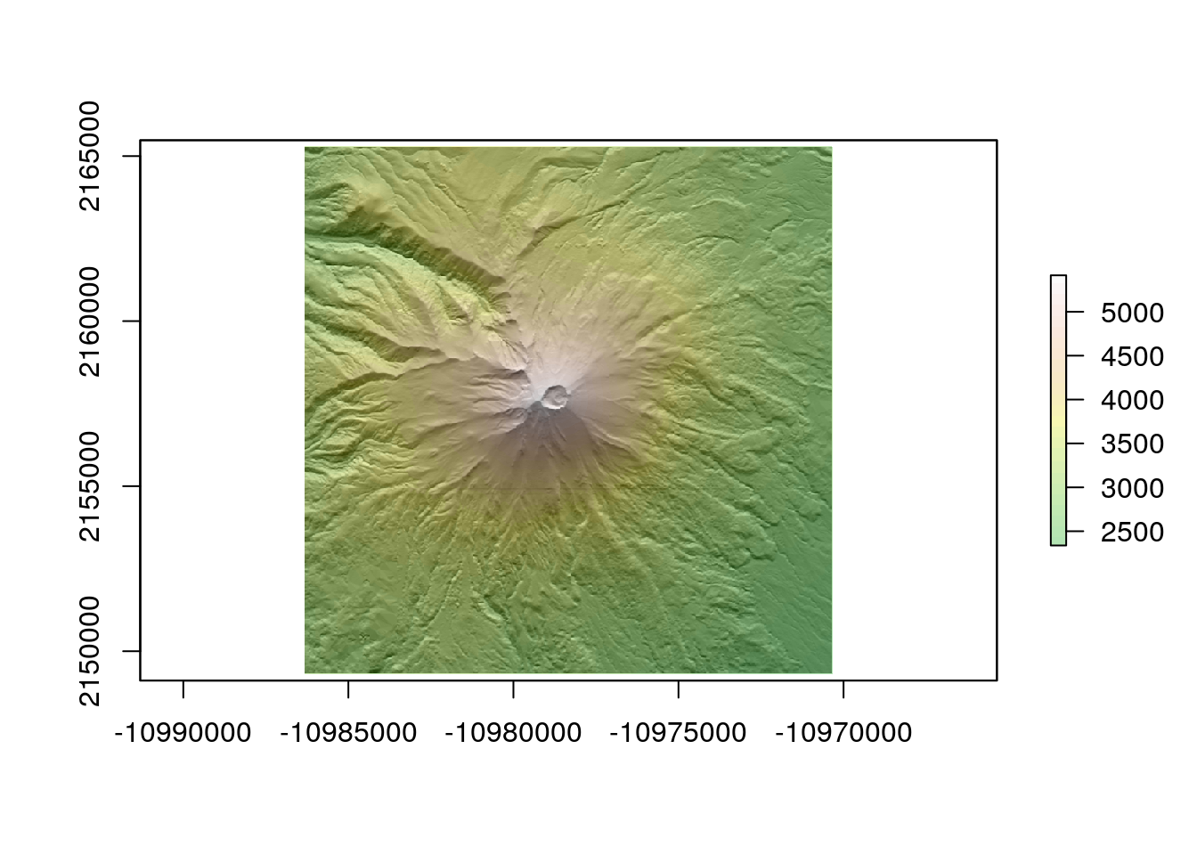

writeRaster(elev,file="rasters/volcanoes/popocateptl.tif",overwrite=TRUE)

10.2.9 Another volcano using the same code.

lon<--99.756
lat <-19.1
radius<-8000

pnt<-data.frame(id=1,x=lon,y=lat)
pnt<-st_as_sf(pnt,coords=c("x","y"),crs=4326)
pnt %>% st_transform(3857)%>% st_buffer(radius) -> circle
elev <- get_elev_raster(circle, z = 12,clip="bbox")
elev <- projectRaster(elev, crs=st_crs(circle)$proj4string)

sloper<-terrain(elev, opt='slope', unit='radians')
aspectr<-terrain(elev, opt='aspect',unit='radians')
hillshade<-hillShade(sloper,aspectr,angle=5)
plot(hillshade, col = gray(0:100 / 100), legend = FALSE)
plot(elev, col = terrain.colors(25), alpha = 0.3, legend = TRUE, add = TRUE)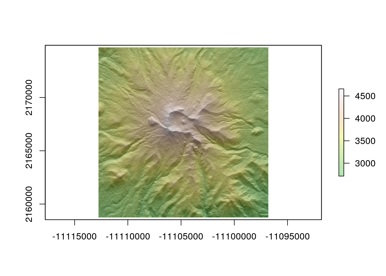

writeRaster(elev,file="rasters/volcanoes/nevado_toluca.tif",overwrite=TRUE)

10.2.10 Load the results to postgis for work in QGIS

query<-"drop schema if exists volcanoes cascade;create schema volcanoes"
dbSendQuery(conn,query)
#> <PostgreSQLResult>

srid<-3857
db<-"gis_course"
path<-"rasters/volcanoes"
nms<-dir(path, pattern="tif")

fls<-paste(path, nms,sep="/")
tbls<-paste("volcanoes",gsub(".tif", "", nms),sep=".")


for(i in 1:length(fls))
{
com<-sprintf("PGPASSWORD=gis_course123 raster2pgsql -d -s %s %s %s | PGPASSWORD=gis_course123 psql -h postgis -U gis_course -d %s",srid,fls[i],tbls[i],db)
system(com)
}

dbDisconnect(conn)
rm(list=ls())
lapply(paste('package:',names(sessionInfo()$otherPkgs),sep=""),detach,character.only=TRUE,unload=TRUE)

10.3 Using QGIS

Conducting some forms of terrain analysis is more natural in the visual GUI provided by QGIS than in R. In particular, finding the right parameters for analytical hillshading can require trial and error in a desktop GIS. So using the strengths of the two different approaches makes sense here.

The layers that were saved into the vocanoes schema from R will show up in the db manager of QGIS after refreshing the connection. They can be loaded into the canvas by clicking on them from the db manager.

Action

1. Start a new project to view the volcano data.
2. Set the project CRS to EPsg 3857 (Web mercator) before loading any layers.
3. Open the db manager and load the volacanoes.
4. Add some base maps and push them below the DTMs.
5. Try running some analytical hill shading. If you make a hillshading layer semi transparent you can vsualise the results with the basemaps. Experiment with this.

Raster layers do not appear in the postgis browser side bar. You need to look for them in the data base manager. The capability to store raster data within a postgis data base was developed much later than the functionality with vector data. Although it is useful to be able to store and process rasters within postgis it is more difficult to use a database for raster work and a database arguably offers rather fewer advantages. So there is still less emphasis placed on this aspect of Postgis. Geoservers and mapservers are still more conventional tools for sharing rasters online.

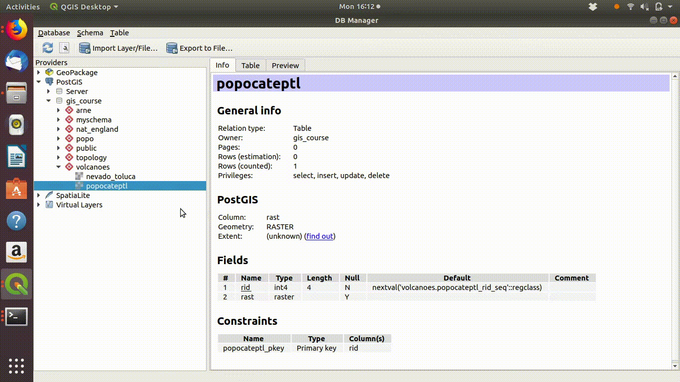
Figure 10.3: The raster layers that were saved from R into the postgis schemas do not show up on the postgis connection browser tab. However they can be found by the data base manager. Clicking on the layer loads the raster into the canvas. This operation can take a few seconds, as raster layers tend to require more memory than vector layers, even for small areas.

Producing derived raster layers from any digital elevation model in QGIS is easy. Simply find the options under the raster menu analysis tag. It is worth experimenting with these. You can also experiment with different ways of shading the results visually.

A useful trick when looking at digital elevation models is to install the qgis2threejs plugin. At the time of writing this plugin still offers the best way of producing three dimenensional visualisations in QGIS (there is a native 3d map view found under the view menu which may be worth experimenting with, but it has been unstable in early versions).

Action

1. Place a base map or a derived layer that you want to visualise in 3d at the top of the layers panel.
2. Open the QGIS2threejs exporter plugin.
3. Choose the volcano DEM as shown in figure 10.4
4. Experiment!

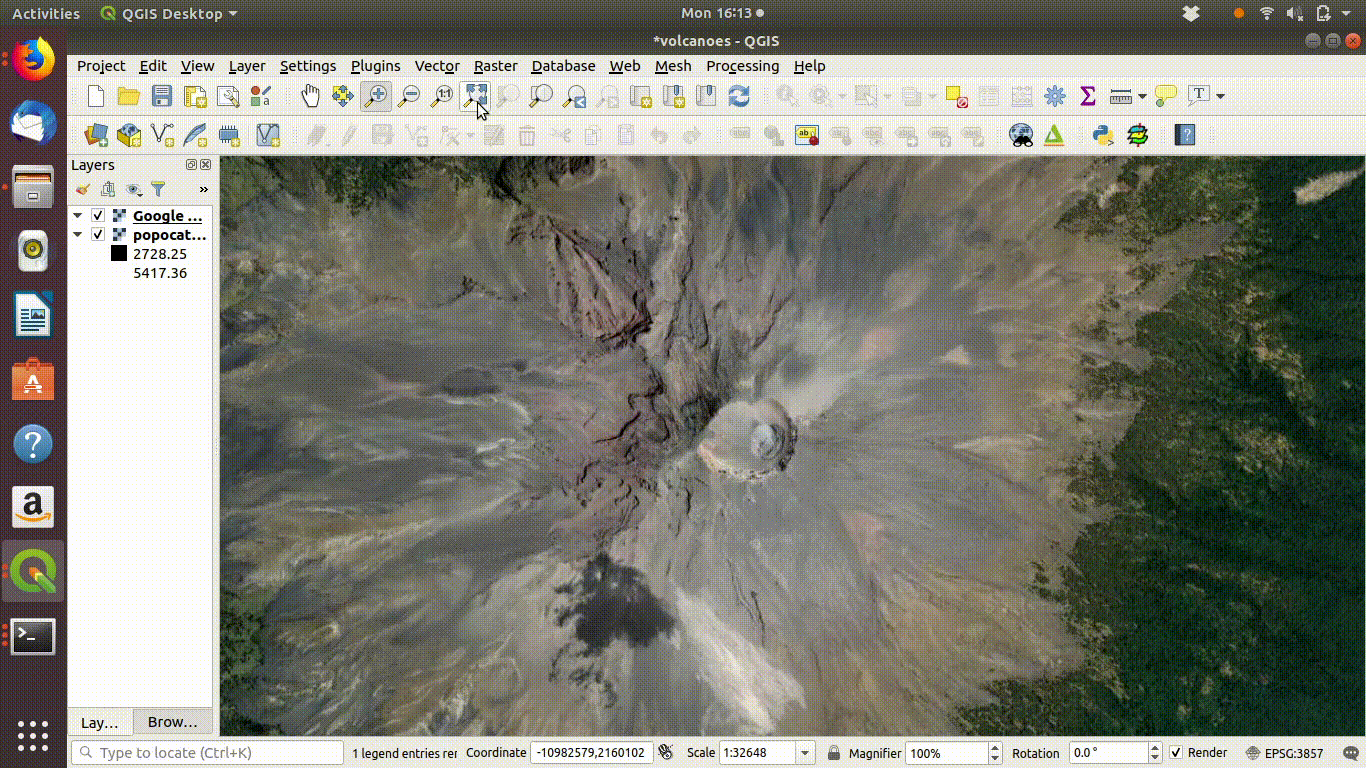
Figure 10.4: Using the Qgis2threejs exporter plugin to visualise Popocateptl vocano. The image can be rotated and zoomed into using the mouse and keypad. Clicking in the image shows the coordinates of the points.

10.3.1 Using the DSM for three dimensional visualisation

Experimenting with the QGIS2threejs plugin is quite easy and intuitive so there is no need for detailed instructions here. It is worth mentioning that if the Lidar derived digital surface model is used with a satelite image draped over it the tree canopy can be visualised as shown in figure 10.5

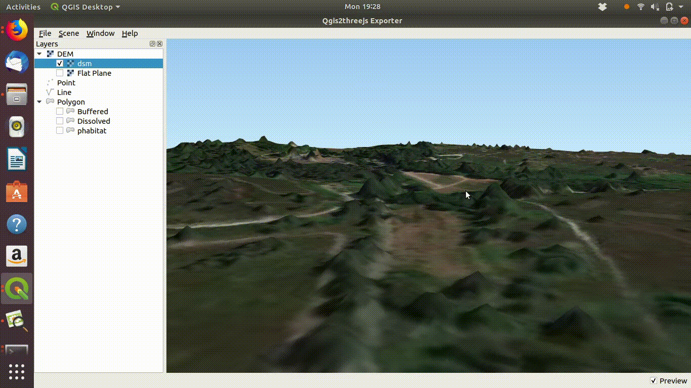
Figure 10.5: Using a digital surface model with the threejs visualisation. This shows the way the DSM is linked to the point cloud as visualised in ef@(fig:lidar1). Notice that if you zoom into the trees they will tend to appear as cone shapes, as the smoothed surface of the dsm will drop away from the highest point of the tree in a rather unnatural fashion. However the visualistion confirms that the lidar layer and the high resolution satelite layers match.