Section 7 Spatial queries

7.1 Concepts

Analysing the spatial relationships between objects is a major aspect of all GIS work. There are three common objectives behind running spatial queries.

1. Extracting subsets of data based on spatial relationships. For example, finding all the calcareous grassland that falls within the county of Doset.
2. Analysing distances between objects numerically. For example, what is the distribution of distances to the nearest road of calcareous grassland patches in Dorset? How much of the grassland can be considered to be part of a road verge?
3. Forming new geometries based on spatial relationships.

This is a very broad subject area. There are multiple ways that spatial SQL can be used within a postgis to work on large data tables and combinations of large data tables. Spatial queries do not have to return spatial layers. Some of the questions may involve calculating derived quantities based on spatial relationships.

The first type of queries are probably the simplest conceptually but the least interesting in other respects. They do not result in any new data or analytical results. However subsetting spatial data to a local site is a very common first step in any analysis.

7.2 QGIS

7.2.1 Quick and easy spatial subsetting

The simplest, and often the quickest, way to obtain a subset of a large data set for analysis at a local level in QGIS does not involve any sql at all. It is simply to zoom to the extent of the area you are interested in, load the data you need from the postgis data base (or from a WCS layer, see section 14.2.1.3 ) then simply save the layers locally, but only saving features that intersect with the visual map extent. This is in effect a spatial query.

As you might use this example in your own project do remember that all saved data should be placed in either the same folder as the project file, or a folder above this in the BU system..

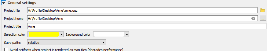
Figure 7.1: Always check your paths carefully on the BU system. Look in the project properties and set the projects home folder to the folder that contains your data. Don’t let the data and the project file become separated or you may not be able to restore the project easily. Notice that the save paths are relative by default, which means folders above the project file position will be recgnised, but those below may not. Take care

Action

Let’s assume we are interested only in looking at data around Cranbourne. Let’s very quickly subset all the calcareous grassland prority habitats and gbif records of blue butterflies stored on our data base to that area.

1. Load the blue butterfly data layer by clicking on it. This is a large layer, but renders quickly as the data are simply points.
2. Zoom out to see the extent of the data

Figure 7.2 shows this in action.

Figure 7.2: Loading the layer called blues from the postgis data base. The layer has point locations for all the gbif records for adonis and chalk hill blue butterflies. Zooming out shows the scale

Action

The next steps are to zoom in to a study area extent. It is convenient to set an extent as a bookmark in QGIS so that it is easy to return to.

See Figure 7.3 to watch the steps in action.

Figure 7.3: Zooming to the study area. Notice the use of a bookmark to hold the extent. These can be set using the bookmark menu on the top of the menu bar. Bookmarks are kept in the project file and can be used to zoom back to exactly the same map extents.

Action

Now all that is needed is to save the two files locally (within your project folder or in a path above it).

1. Right click the layer name
2. Choose export
3. Select the options to save the layer. Give the file a new name to prevent confusion.
4. Set the extent to the map canvas extent. This is the vital step.
5. Remove the layers that were loaded from the postgis data base, as these are no longer needed for the local project
6. Save the project
7. You can now work on the data anywhere, including off campus if you copy the folder with the data contained.

See Figure 7.4, figure Figure 7.5 and Figure 7.6 to watch all the steps in action.

Figure 7.4: Save the layers locally. Make sure that you set the extent being saved to the map canvas extent. Save under a different name. Then remove the postgis layer.

Figure 7.5: Removing the postgis layers.

Figure 7.6: Repeating and tidying up

This is a very simple way of saving layers to a desktop GIS project that only contain the local features. The advantage is that the work flow is very quick and simple. The disadvantage is that it is not strictly reproducible.

7.2.2 Using SQL

To illustrate the use of spatial queries in QGIS to subset layers we can also look at a few other useful features of QGIS in conjunction with postgis. This approach enhances reproducibility by saving a definition of the study area that can be used by others and passed from QGIS to R.

All postgis data base users are assigned a user name. In this course you can share a common user name (gis_course). In a real life project there would usually be a private user name for each user. These users can add data to either the public schema, or to their own private schemas. Other users cannot automatically access private schemas without permission.

If a new layer is digitised as a scratch layer in QGIS it can be transfered intto a user’s schema and used to define a study region boundary. Although this involves a little more work than just zooming to an area, there are some big advantages in doing this. If the study region is a complex shape, or if it is a disjunct set of areas, the digitised polygon can capture this complexity. The persistance of the layer on the server also allows the layer to be easily passed through into R without any need to transfer any files. The study area can also be saved and used by others.

The steps needed are ..

1. Digitise a polygon (or polygons) representing the area of interest.
2. Load this geoemtry into the data base in a personal schema.
3. Use the polygon(s) within a spatial query to subset the layers of interest.

Action step 1

Define a temporary scratch layer for the polygon.

1. Click on layer then add layer.
2. Give the layer a name
3. Define the geometry type as polygon.
4. Make sure the CRS is set to 27700 (British National Grid)

Figure 7.7

Figure 7.7: Starting a temporary scratch layer: Click on layer then add layer.Give the layer a name.Define the geometry type as polygon. Make sure the CRS is set to 27700 (British National Grid)

Action step 2

Draw the polygon(s).

1. Click on the pencil symbol to switch on editing.
2. Click on the polygon symbol to start drawing.
3. Draw a polygon around the study area. This can be as precise or rough as needed for the job at hand.
4. Right click to complete the polygon
5. Switch off the editing to save the polygon.

Figure 7.8 shows these steps

Figure 7.8: Drawing a new polygon: Click on the pencil symbol to switch on editing.Click on the polygon symbol to start drawing.Draw a polygon around the study area. This can be as precise or rough as needed for the job at hand.Right click to complete the polygon:Switch off the editing to save the polygon.

Action step 3

1. Save the polygon and stop editing.
2. Open the db manager menu.

Figure 7.9 shows these steps

Figure 7.9: Saving the polygon when stopping editing

Action step 4

1. Create a new schema. The name of the schema would be associated with the user, but for the purposes of this demo we’ll just call it “myschema”
2. Import the scratch layer into the schema. Give the layer a name.
3. The polygon is now saved within the data base so it can be used in a spatial query.

Figure 7.10 shows these steps

Figure 7.10: Creating a new schema called myschema. The scratch layer in the canvas is imported with the name cranborne

Action step 5

1. Now write out an sql query. The query will look like this

select c.* from calc_grass c, myschema.cranborne my where st_intersects(my.geom,c.geom)

2. The logic of the query is explained below 7.2.2.1
3. The query combines two tables. The target table for subsetting is calc_grass.
4. The simple table containing the study area polygon (myschema.cranborne) is used to subset the target table spatially.
5. All the fields of the target (select c.*) are chosen based on the where clause.
6. The where clause uses st_intersects to select geometries that intersect. st_intersects(my.geom,c.geom)

Figure 7.11 shows the query being written out in the db manager.

Figure 7.11: Writing an SQL query to spatially subset the calcareous grassland layer to the study area.

Action step 6

1. Run the query
2. Load the results into the canvas.
3. The result is the target layer clipped to the digitised polygon. The layer can then be saved locally for further analysis.

Figure 7.12 shows the query loaded into the canvas.

Figure 7.12: Loading the results of the spatial query into the canvas

7.2.2.1 Breaking down the query

The query is quite simple to understand. The first line selects all the fields from the calc_grass table. Notice that the table is given an alias of c to avoid having to type out the full table name. The polygon used to clip the layer is myschema.cranborne. This is given an alias of my. Then the where clause uses the st_intersect operator to define which of the geometries from the target layer are within the polygon. An intersect operator works when a geometry is either within or touching another geometry.

select c.* from calc_grass c, myschema.cranborne my where st_intersects(my.geom,c.geom)

7.3 Spatial queries in R

require(sf)
require(tmap)
require(giscourse)
require(mapview)
conn<-connect()

7.3.1 Sharing the results of polygon capture in QGIS

A key feature of using a postgis data base as a back end for doing GIS is the fact that layers can be shared between the QGIS desktop and R, even when the actual analyses are being run on different computers with different file systems.

In the example above a polygon was captured that represented the rough boundaries of an example focus area.

This can be quickly visualised in R by piping the query result into mapview.

poly_sql<-"select geom from myschema.cranborne"
st_read(conn, query=poly_sql) %>% mapview()

OK, this is the result of digitising in QGIS. So we can now extract data that overlaps the area and use it in R. This time let’s get all the heathland in the study area, not the calcareous grassland. To do this we combine two queries in one.

The query to extract heathland is written as

select main_habit, geom from ph_v2_1 where main_habit ilike ‘%heath%’

poly_sql<-"select geom from myschema.cranborne"
heath_sql<-"select main_habit, geom from ph_v2_1 where main_habit ilike '%heath%'"

7.3.2 Joining using sprintf.

Subqueries are placed in brackets within a main query and given an “alias”.

We can join the two subqueries using the sprintf trick shown in the tips and tricks section 17.11

sprintf("select * from (%s) c, (%s) h where 
st_intersects(c.geom,h.geom)",poly_sql,heath_sql)
#> [1] "select * from (select geom from myschema.cranborne) c, (select main_habit, geom from ph_v2_1 where main_habit ilike '%heath%') h where \nst_intersects(c.geom,h.geom)"

The query follows the same logic as shown for spatial queries in QGIS.

select * from myschema.cranborne c, (select main_habit, geom from ph_v2_1 where main_habit ilike ‘%heath%’) p where st_intersects(p.geom,c.geom)

This is the result of running the query. The map shows heathland within the study area.

query<-sprintf("select * from (%s) c, (%s) h where 
 st_intersects(c.geom,h.geom)",poly_sql,heath_sql)
heathland<-st_read(conn, query=query)
mapview(heathland)

7.3.3 Arne example

We are going to use the RSPB reserve at Arne as an example site for some of the techniques shown later in this book. So let’s get the priority habitats for the SSSI.

query<-" select h.* from 
(select * from sssi where sssi_name like 'Arne') s,
ph_v2_1 h 
where st_intersects(h.geom,s.geom)"
habitats<-st_read(conn, query=query) 

habitats<-st_zm(st_read(conn, query=query) ) ## Note that sometimes the st_zm operator is needed to turn geomtries in the right format
qtm(habitats,fill="main_habit") +tm_style("classic")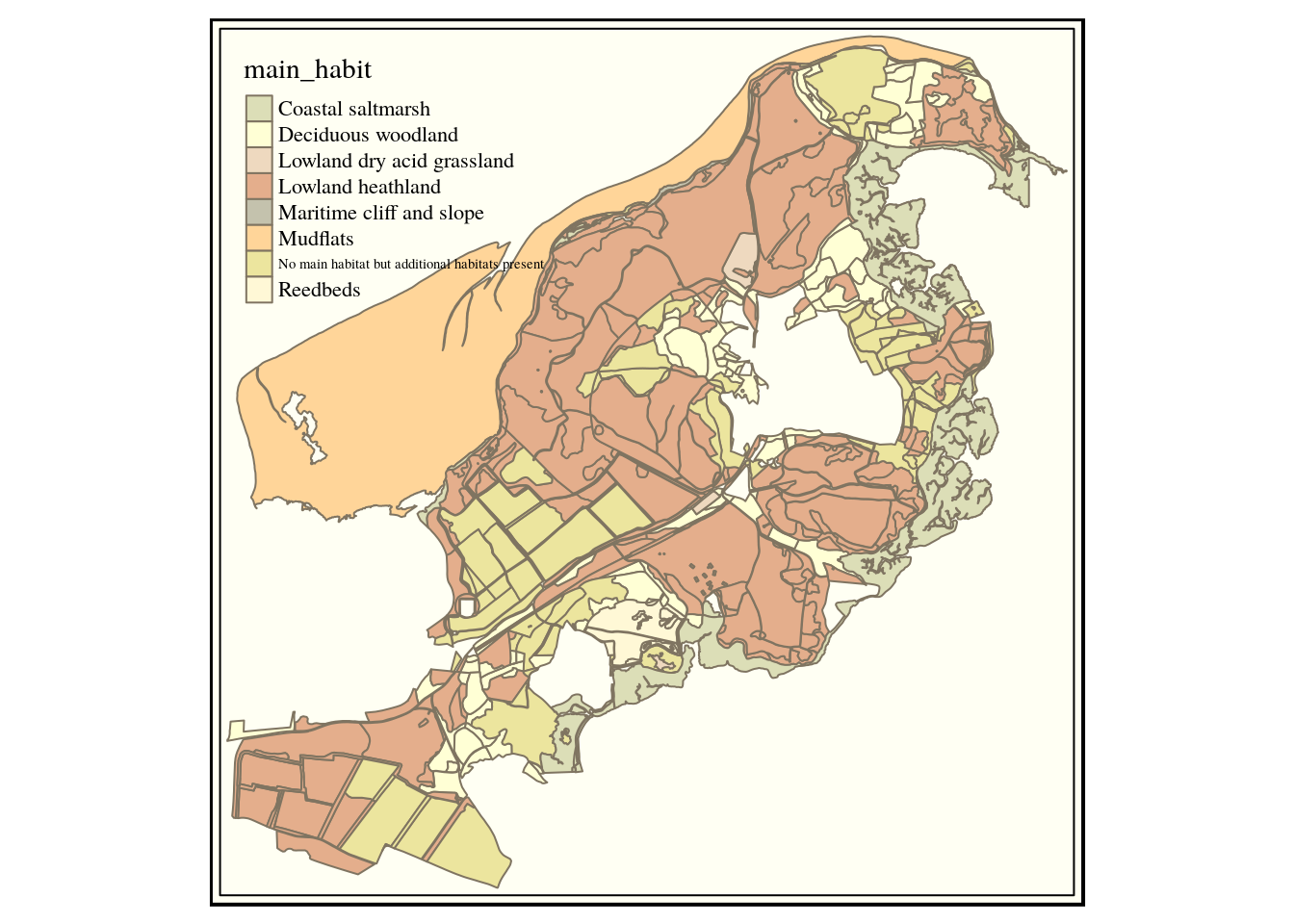

This looks oK, but we might want to tidy it up a bit more by just clipping to the sssi.

7.3.4 Forming new geometries

The st_intersects operator that we have used extracts all geometries that share space. If the geometries extend beyond an area of interest this can produce results that we don’t want. Let’s just choose the elements that fit within the sssi and cut out any parts of a polygon that falls outside. This is known as clipping. To do this requires a slightly more complex query. The first line of the query above is altered to read

select main_habit mhabitat, s1habtype,s2habtype,s3habtype habitat,st_intersection(h.geom,s.geom)

This works by forming a new geometry based on the intersection between the habitat geometry and the sssi geometry. Note that this differs from the st_interscts operator as the latter just selects the intersecting geometries but does not form a new geometry. When the two are placed together we are clipping the layers. This is a form of geoprocessing. See section 9

As a new geometry is formed we can’t use a * in the first line to select all the fields in the habitat layer, as this would produce two geometries. So we need to write out all the fields we want to return. We’ll just choose the fields we are actually going to use in subsequent analyses in order to simplify the layer.

query<-" select main_habit mhabitat, s1habtype,s2habtype,s3habtype habitat,
st_intersection(h.geom,s.geom) geom 
from (select * from sssi where sssi_name like 'Arne') 
s,ph_v2_1 h 
where st_intersects(h.geom,s.geom)"
habitats<-st_read(conn, query=query) 

qtm(habitats,fill="mhabitat") +tm_style("classic")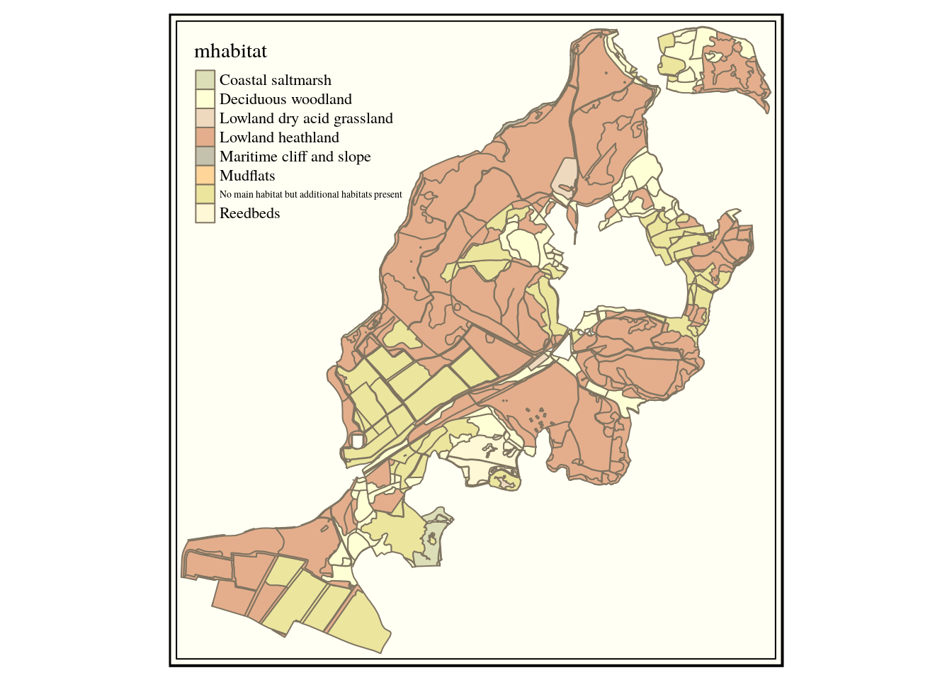

7.3.5 Forming a new schema and adding tables

As we are going to work with this layer further we probably won’t want to keep running the query every time we need it. We can also place some other useful layers in a schema for the study area. So we’ll set up a schema from R and add a table to it.

## Be very careful when using drop cascade as this wipes out any information in the schema if it does already exist. Make sure this is what you really intend to do.
query<-"drop schema if exists arne cascade; 
create schema arne;"
dbSendQuery(conn,query)
#> <PostgreSQLResult>

Now we can form a table. Notice that it is always a good idea to add row numbers to a table as a unique identifier. This is needed to load a query in QGIS and other software. See tip 17.7 . We can do this by adding row_number () over () to the query.

query<-"create table arne.phabitat as
select row_number() over() id, 
main_habit mhabitat, 
s1habtype,s2habtype,s3habtype,
st_intersection(h.geom,s.geom) geom 
from (select * from sssi where sssi_name like 'Arne') 
s,ph_v2_1 h 
where st_intersects(h.geom,s.geom)"
dbSendQuery(conn,query)
#> <PostgreSQLResult>

Queries like this should be built up step by step. Although the sql appears complicated and hard to read, each individual step is quite simple.

7.3.6 Using OSM vector data

The information in the open street map basemaps that can be used for webmapping can be downloaded and placed in a postgis data base as vector layers. This can be useful if operations such as calculating distances from features visible on the basemap is required.

The manner in which information was collected for OSM evolved over time, so unfortunately the data format for OSM layers is notoriously unconventional making the source rather difficult to use. For example the word “way” is used in osm layers to refer to the geometry column. Many of the columns are blank and a tagging system is used when designing more complex queries in postgis.

Ot is useful to obtain vectors representing features that cnn be seen on the basemap. So, as an example of OSM usage let’s try to find all the tracks, paths and bridleways in the Cranborne area.

The column holding roads, paths and other rights of way is rather strangely, called highways. This line makes a quick searchable table in R to find what it holds.

dbGetQuery(conn, "select distinct highway from dorset_line") %>% 
  data.frame() %>% DT::datatable()

OK. This is a little bit awkward as there are multiple possible choices, but this query should do the trick

query<-" select osm_id,highway,st_intersection(way,geom) geom from 
(select * from myschema.cranborne) s,
(select * from dorset_line where 
highway in ('bridleway' , 'footway' ,'pedestrian' 
, 'track', 'path' ) )l
where st_intersects(way,geom)"
st_read(conn, query=query) %>% mapview()

The following query will find roads and paths that intersect the sssi at Arne.

arne_sssi<- st_read(conn, query="select * from sssi where sssi_name like 'Arne'")
query<-" select osm_id,highway,way from 
(select * from sssi where sssi_name like 'Arne') s,
dorset_line l
where st_intersects(way,geom)"
paths<-st_read(conn, query=query) 

qtm(paths)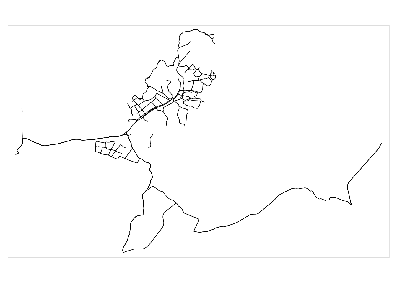 

The issue is that the paths and roads that intersect the sssi extend beyond the limits. To change this requires the formation of a new geometry again using st_intersection().

query<-" select osm_id,highway,st_intersection(way,geom) geom from 
(select * from sssi where sssi_name like 'Arne') s,
dorset_line l
where st_intersects(way,geom)"
paths<-st_read(conn, query=query) 
qtm(arne_sssi) + qtm(paths)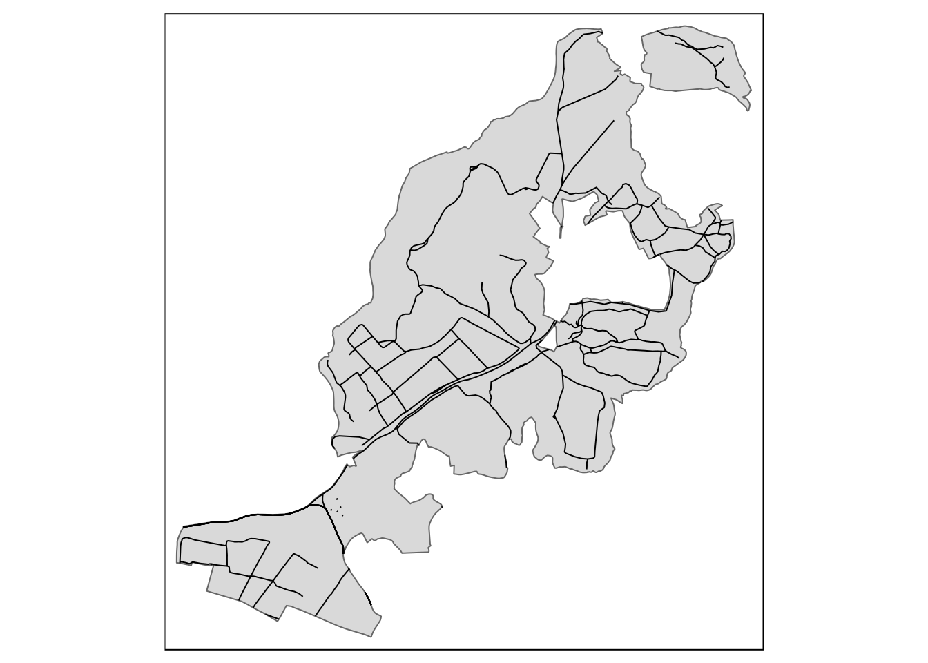

OK. so let’s put this into the schema too.

query<- "create table arne.paths as 
select row_number() over() id, osm_id,
highway,st_intersection(way,geom) geom 
from 
(select * from sssi where sssi_name like 'Arne') s,
dorset_line l
where st_intersects(way,geom)"
dbSendQuery(conn, query)
#> <PostgreSQLResult>

7.3.7 Quick and easy spatial queries using Geocoding

The equivalent of the operation shown in QGIS involving zooming and clipping can also be used in R. To make it simpler I’ve included a convenience function in the giscourse package. So if you can write out a query based on an attribute it can be applied only on an area of the table. For example, to obtain all the grazing marsh habitats 1km from the centre of Wareham.

require(giscourse)
query<-"select * from ph_v2_1 where main_habit ilike '%grazing%marsh%'"

st_zm(dquery("Wareham",query =query,1000)) %>% mapview(zcol="main_habit")