Section 13 Species distribution analysis
13.1 Concepts
Producing maps that represent the distribution of species is a central theme in Biogeography. Showing where a species occurs and where it does not, on a map may seem simple. In fact it is a complex task. In some respects this complexity is conceptual in nature. In a world in which maps can be zoomed to any level of visual resolution what does it mean to use a map that shows that a species may be present? Would you expect to actually find evidence that the species occurs at any point within the distribution map? How can the distribution of mobile organisms be mapped? How can we map cryptic organisms whose presence goes largely unnoticed? The fact that a model is based on some aspects of a species requirements assumes that these requirements are fully, or partially, met at a broad scale. However is can never really predict a species presence at a give site. Analysing a species distribution is an iterative process that requires multiple analyses at multiple spatial scales.
13.2 Using R and the dismo package
There is really little point in trying to implement a species distribution analysis in QGIS. It is much easier in R since the raster and dismo packages were made available.
require(dismo)
require(sf)
require(mapview)
require(tmap)
require(RPostgreSQL)
require(dplyr)
library(raster)
library(rgdal)
data(World)
mapviewOptions(basemaps =c("OpenStreetMap",
"Stamen.TonerLite", "Esri.WorldImagery",
"Esri.WorldShadedRelief",
"Stamen.Terrain"))
conn <- dbConnect("PostgreSQL", host = "postgis",
dbname = "gis_course" ,user = "gis_course",
password = "gis_course123")13.2.1 Getting records from gbif
The dismo package has a really useful function for pulling down all the available records for a species from GBIF.
We’ll get the records for the Adonis blue butterfly the Chalkhill blue and their common host plant Horseshoe vetch.
The code below has been run through but it takes at least three hours to obtain all the records. We only want to repeat the exercise occasionally in order to update the records from gbif. The code is provided for reference but it has been commented out here to prevent accidentally running it.
# d<-gbif("Hippocrepis","comosa",geo=TRUE) # get all records of Horseshoe vetch
# d<-d[!is.na(d$lon),] # Take out blanks
# vetch<-st_as_sf(d,coords=c("lon","lat"),crs=4326) # make sf
# d<-gbif("Polyommatus","coridon",geo=TRUE) # get all records of Chalkhill blues
# d<-d[!is.na(d$lon),]
# chil<-st_as_sf(d,coords=c("lon","lat"),crs=4326)
# d<-gbif("Polyommatus","bellargus",geo=TRUE) # get all records of Chalkhill blues
# d<-d[!is.na(d$lon),]
# adonis<-st_as_sf(d,coords=c("lon","lat"),crs=4326)13.2.1.1 Simplifying the data
GBIF provides records that use the Darwin core set of column headers. Unfortunately there are different numbers of fields for each species and the number varies from 140 to 156. Many of the fields contain repeated information that is only useful for printing out a formal taxonomic record. There is also a lot of blank space in the records. For analysis purposes we only really need the species name and perhaps the date of observation. So we’ll clean these records up, simplify them and then place them in the data base.
# First change all the names to lower case
# names(vetch)<-tolower(names(vetch))
# names(chil)<-tolower(names(chil))
# names(adonis)<-tolower(names(adonis))
# library(dplyr)
# # Now choose only the most useful fields.
# useful<-c("genus", "species", "coordinateuncertaintyinmeters", "country","eventdate")
#
# vetch %>% select(useful) -> vetch
# adonis %>% select(useful) -> adonis
# chil %>% select(useful) -> chilNote that if all the field names match up we could build a single table for all gbif records many species. If we then want to extract a specific records we can filter on species or genus. This is more efficient than making a table for butterflies and another for plants. However to simplify matters for the purpose of the course a simple table called blue has been produced for just the butterflies. That was just because it is easier to use directly in QGIS without running a filtering query.
13.2.1.2 Writing the records to postgis
# blues<-rbind(adonis,chil)
# gbif<-rbind(adonis,chil,vetch)
#
# st_write(blues, conn)
# dbSendQuery(conn, "create index blues_ind on blues using gist (geometry)")
#
# st_write(gbif, conn)
# # Make indices
# dbSendQuery(conn, "create index gbif_ind on gbif using gist (geometry)") dbSendQuery(conn, "create index gbif_names_ind on gbif (species)")
# dbSendQuery(conn, "create index gbif_genus_ind on gbif (genus)")13.2.2 Looking at the records
Now the gbif records are in the data base we can easily filter them to the UK and then visualise them.
query<-"select geometry,species from gbif where country = 'United Kingdom'"
records<-st_read(conn, query=query)However there is a slight problem visualising the points using mapview. There are 110,000 points, as we can see if we ask for the dimensions of the data.
dim(records)
#> [1] 221922 2While this will load into mapview these are a lot of points to show on a single map and so the rendering is very slow. So let’s just filter out a random set of two thousand for the moment.
query<-"select geometry,species from
gbif where country = 'United Kingdom'
order by random() limit 2000"
st_read(conn, query=query) %>% mapview(zcol="species", burst=TRUE) -> rec_map
rec_map13.2.3 Aggregating counts to a grid
When looking at patterns of occurrence the actual values of the counts are not very informative. Some sites are very regularly collected or observed but the numbers of observations don’t necessarily indicate abundance. They may indicate activity of collectors or monitoring programs. Presence or absence is more useful and the forms the basis of a standard empirical range map.
Traditionally in the UK counts of observations falling within the conventional ordinance survey 5km grid squares have been used for mapping species ranges. The OS grid 5km tiles are loaded into the postgis data base under the table name os5km.
Joining the point data with the grid is a job that postgis does very quickly and efficiently. However, writing out the appropriate query is not a task for a beginner in spatial sql. It involves a few steps and some care. Queries such as these are best built up step by step and tested in the db manager query builder in QGIS (or a Postgresql client such as PgAdmin) before pasting into the R code. There are two steps to the query.
- The coordinate reference system for the OS5km layer is EPSG 27700. However the gbif records are held as lat long EPSG 4326, as they are potentially global. See section 5. So if an intercept query used the records in this form it would return no results. The best way to resolve these issues is to keep all data on a data base in the same projection. However in this case it would not be logical to do so. It is possible to transform “on the fly” within the structure of a single query. However this leads to queries that run very slowly as they can’t use spatial indexing. So the best way to handle this issue is to build a new table in EPSG 27700 for the gbif records and index it.
- The query then uses a powerful feature of SQL to aggregate the data. This is grouping. If one or more fields are included in a grouping clause in a query then stats such as mean, maximum, count etc. can be calculated on a field that is not included in the grouping. So in this case we can group on species and grid square then take the count.
- As this result may be useful in QGIS we will then form a table from it when running the query in R so that it does not have to be run again. An index should be placed on tables for speed.
## This code implements the grid count query
query<- "drop table if exists gbif_27700 cascade;
drop table if exists gbif_gridded cascade;
create table gbif_27700 as
select species, st_transform(geometry,27700) geometry from gbif;
create index gb_27700 on gbif_27700 using gist(geometry);
create table gbif_gridded as
select row_number() over () id,
tile_name, species,count(species),geometry from
(select gb.species,os.geometry,tile_name from
os5km os,
gbif_27700 gb
where st_intersects(os.geometry,gb.geometry)) s
group by species,geometry,tile_name;
create index gbif_grid_ind on gbif_gridded using gist(geometry);"
# dbSendQuery(conn,query) ## Implements the query when uncommented13.2.4 Visualising the gridded data
The gridded table will only contain OS 5km grid squares with one of the three species of interest.
gridded<-st_read(conn,query="select * from gbif_gridded")
gridded$occurence<-(gridded$count>0)*1 # Make a column of ones and zeros
mapview(gridded,zcol="species",burst=TRUE) -> grid_map
grid_map13.2.5 Testing the association between species occurrences
That an association at a national scale between the occurrences of all three species occurs is very clearly evident from the map. There is nothing much to be gained by testing this statistically. The two butterfly species depend on the host plant, so their distribution much follow. However we might be curious with regards to the local co-occurrences of Adonis and Chalkhill blues. These have been recorded within the subset of grid squares that have been selected as containing at least one of the three species of interest, i.e.including the host plant. So, is a grid cell with a record of an Adonis blue more or less likely to have a record of a chalkhill blue given that the cells all have appropriate habitat within them.
In this case it is useful to turn the data frame into a wide, sites by species matrix format. This is very simple using the tidyr package.
require(tidyr)
gridded %>% select("tile_name", "species","occurence") %>% st_set_geometry(NULL) %>% spread(species, occurence,fill=0) -> oc_df
gridded %>%
select("tile_name", "species","count") %>%
st_set_geometry(NULL) %>% spread(species, count,fill=0) -> count_dfNow we can produce a contingency table showing the proportions of occurrences and co-occurrences.
round(prop.table(table(oc_df[,3:4]),1) *100,1)
#> Polyommatus coridon
#> Polyommatus bellargus 0 1
#> 0 46.7 53.3
#> 1 17.3 82.7It is quite clear from this that the two species do tend to occur together. The table shows that 83% of grid squares with a record of Adonis blue also have at least one record of the Chalkhill blue. This is clearly highly significant. The chi squared test is just a formality.
chisq.test(table(oc_df[,3:4]))
#>
#> Pearson's Chi-squared test with Yates' continuity correction
#>
#> data: table(oc_df[, 3:4])
#> X-squared = 68.424, df = 1, p-value < 2.2e-16The table approach also gives the absolute area of each combination in square kilometers when multiplied by 25.
round(table(oc_df[,3:4]) *25,0)
#> Polyommatus coridon
#> Polyommatus bellargus 0 1
#> 0 5000 5700
#> 1 1350 6475We might want to check quickly whether the actual counts are also correlated in some respect. The count data is extremely heavily right skewed. Some grid squares contain many thousands of observations. So a formal statistical analysis might use a glm of the negative binomial family to model these data, or a very simple analysis could just use rank correlation. A quick visualisation can be obtained by log transforming the axes (zeros will clearly be lost in the process).
require(ggplot2)
count_df %>%
ggplot(aes(x=`Polyommatus bellargus`,y=`Polyommatus coridon`)) +
geom_point() +
geom_smooth() +
scale_x_log10() +
scale_y_log10()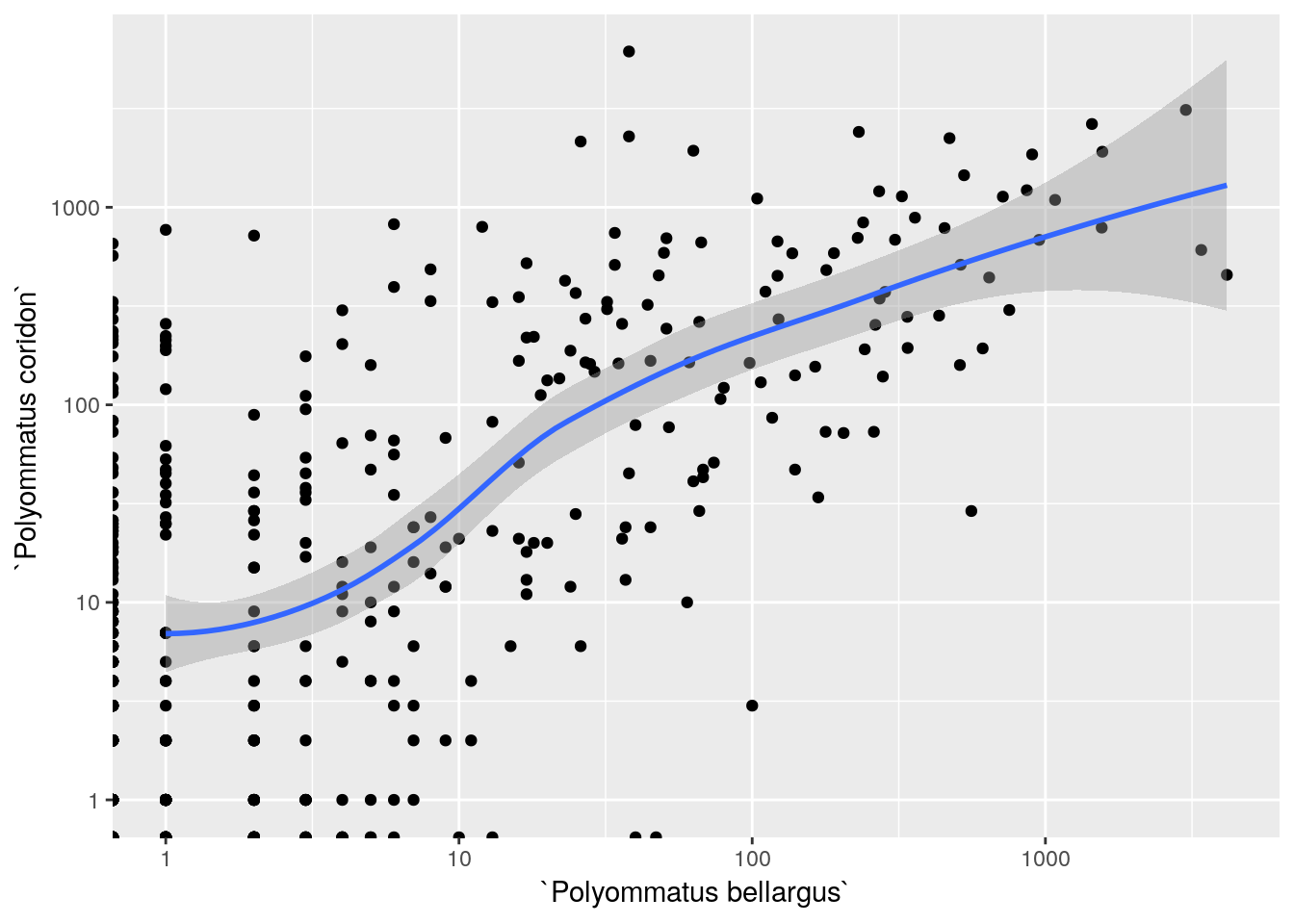
There is a very clear relationship and no need to run a test for it. As this is at least partly the result of observer bias it would not be a particularly useful relationship for modelling purposes. It is clear that grid squares with high numbers of observations of Adonis blue do tend to have high numbers of observations of Chalkhill blues. The reason may need more investigation.
13.2.5.1 Association with geology
The association between both species with their host plant, the horseshoe vetch, is assumed from the start. The key is also in the name of the species. It would be odd if the chalkhill blue was not associated with chalk! Let’s look at this as a map.
We can extract all the areas of chalk or limestone from the bedrock table in the postgis data base which is taken from the British Geological Society maps. http://mapapps.bgs.ac.uk/geologyofbritain/home.html
query<-"select rcs_d,st_simplify(geom,100) geom from
bedrock where rcs_d ilike 'CHALK%' or
rcs_d ilike 'LIMESTONE%'"
chalk<-st_read(conn, query=query)
chalk_map<-mapview(chalk,legend=FALSE)
chalk_map + grid_mapThe association is very clear, although it is not completely perfect. A few records for the vetch fall outside areas with calciferous bedrock. It may be that some localised sites have appropriate conditions outside the broad scale of the underlying geology.
13.2.6 Modelling species distribution using maxent
Species distribution modelling has become very popular with thousands of published papers based on use or discussion of the techniques involved. One of the most used tools is maxent.
https://biodiversityinformatics.amnh.org/open_source/maxent/
Maxent is now open source, which is good news. There are many other algorithms for machine learning that can produce species distribution maps in R. However maxent probably became the tool of choice because it had its own GUI so could be used by non programmers. However it is really much easier to use maxent from R. Learning to get the data into the maxent GUI can take some time. Data transfer from R is simple. The results are the same.
There are many pitfalls in species distribution modelling. In particular the approach used in this example is NOT recommended in a research context. Finding a justifiable model that represents meaningful relationships between climatic factors and species distribution requires very carefull consideration of the species ecology. There are many different options that can be used when building models.
Any species distribution modelling algorithm based only on occurrence points uses some system to generate “pseudoabsences” or background points as a contrast. The algorithm aims to distinguish between these two classes of observations based on the values of input layers.
13.2.6.1 Step 1. Get some occurrence data.
This step is not necessarily as simple as it may seem. Although the points at which the species has been found are registered in the data base, each spatial point may have multiple observations. The points are spatially autocorrelated simply because the species distribution is a spatial phenomena.There are a wide range of choices that can be taken at this point in model building. Here we’ll just use a simple random sample of the available points. Making a different choice may change the final result.
occurence <- st_read(conn,query="select * from gbif
where genus = 'Hippocrepis'
order by random() limit 10000")13.2.6.2 Step 2. Define the area of interest
This is another decision that introduces subjectivity into the model building process. What are we actually trying to define when we use the algorithm to distinguish between areas in which the species occurs and areas in which it does not?. If we allow the algorithm to run on the whole global worldclim layers it should be able to tell us that the species does not occur in the Sahara desert nor the Greenland ice cap. However this is not really useful. Conversely if we define an area around the points that has a very uniform climate the model is not going to distinguish between any areas with species occuring and areas where the species does not. We’ll use a buffer of around 100 km (1 degree) around a convex hull of the presence points here.
limits<-st_convex_hull(occurence) # Make a hull around the points
limits<-st_buffer(limits,1) # Set the area of interest to 1 degree around the points
limits<-as(limits,"Spatial") # Needed as the code uses the older form of R spatial objects.
occurence <- as(occurence, 'Spatial') ## Change to the old spatial class13.2.6.3 Step 3. Choose the predictors
This is another subjective choice. If you want to produce a map that shades in pixels to match the density of the current species distribution it doesn’t matter which layers are chosen as predictors. In fact the easiest, and best, choice for this purpose is to use all available layers. This will allow the algorithm to (over) fit to the current pattern. The challenge that arises is that models are frequently used to predict distributions under novel scenarios. If they are designed to achieve that goal then much more attention is needed. Each predictor should map on to some aspect of the species ecology in a meaningful way. A machine learning aglorithm requires a lot of supervision to work effectively. In this example this supervision is lacking. You may wish to try to include it when carrying out the exercises.
worldclim<-getData(name = "worldclim", var = "bio", res = 5) ## Get all the bioclim layers
future <- getData('CMIP5', var='bio', res=5, rcp=85, model='AC', year=50)
worldclim<-raster::crop(worldclim,limits)
worldclim_future<-raster::crop(future,limits)
# witholding a 20% sample for testing
fold <- kfold(occurence, k=5)
occtest <- occurence[fold == 1, ]
occtrain <- occurence[fold != 1, ]
me <- maxent(worldclim, occtrain, path="maxent")dist_now <- predict(me, worldclim)
names(worldclim_future) <- names(worldclim)
dist_future <- predict(me, worldclim_future)
dist_now[dist_now<0.3]<-NA
dist_future[dist_future<0.3]<-NAlibrary(rnaturalearth)
europe <- ne_countries(continent = 'europe',10)
qtm(dist_now) +
qtm(europe, fill=NULL) +
tm_legend(legend.outside=TRUE)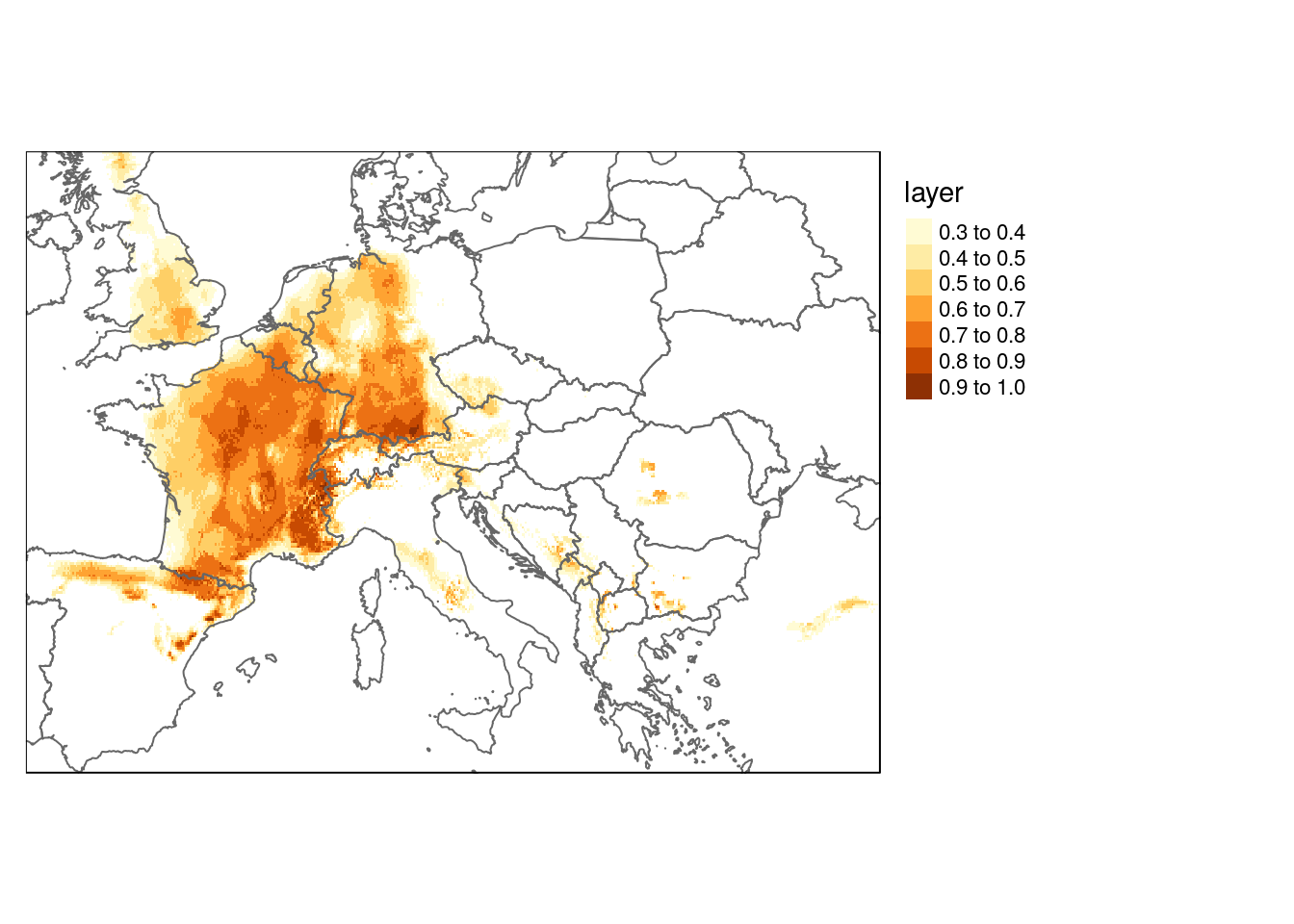
qtm(dist_future) +
qtm(europe, fill=NULL) +
tm_legend(legend.outside=TRUE)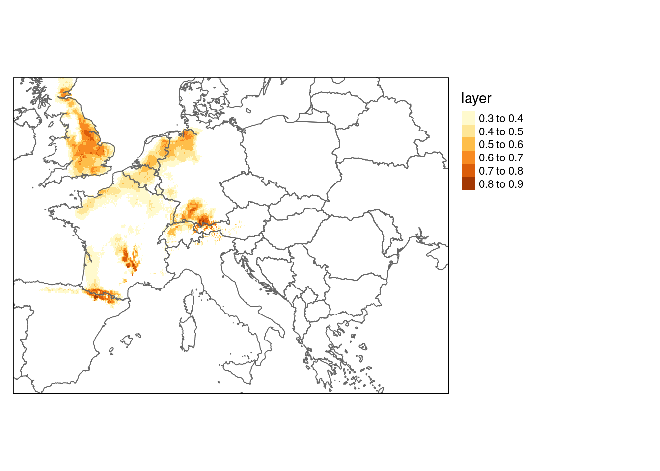
query<-"select st_transform(geom,4326) geom
from bedrock where rcs_d ilike 'CHALK%'
or rcs_d ilike 'LIMESTONE%'"
chalk<- st_zm(st_read(conn, query=query))
bounds<-as(chalk,"Spatial")
dist_now<-raster::crop(dist_now, bounds)
dist_future<-raster::crop(dist_future, bounds)
qtm(dist_now) + qtm(europe, fill = NULL) + tm_legend(legend.outside=TRUE)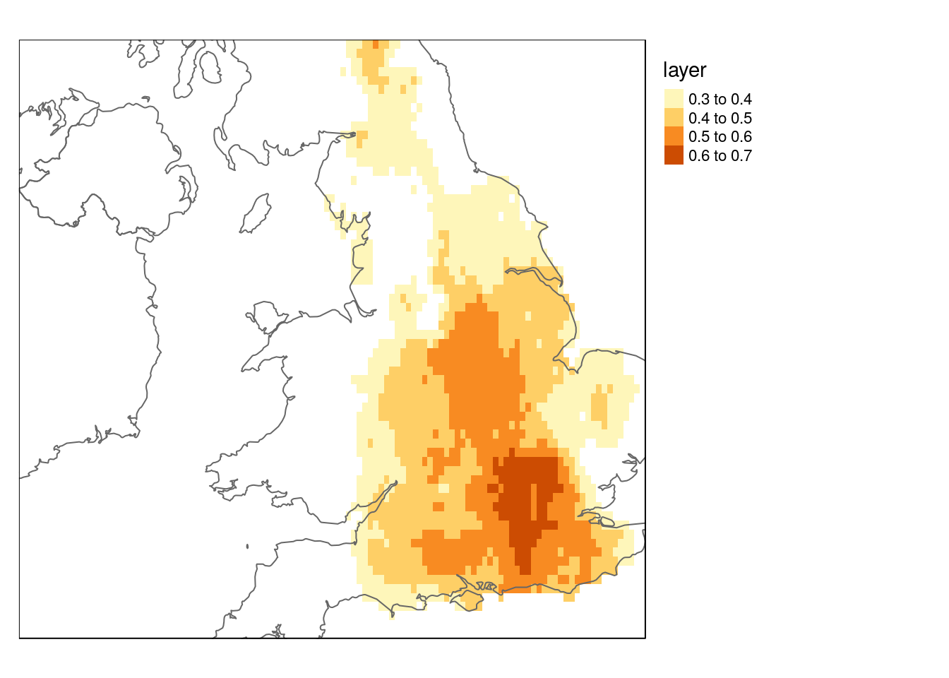
qtm(dist_future) + qtm(europe, fill = NULL) + tm_legend(legend.outside=TRUE)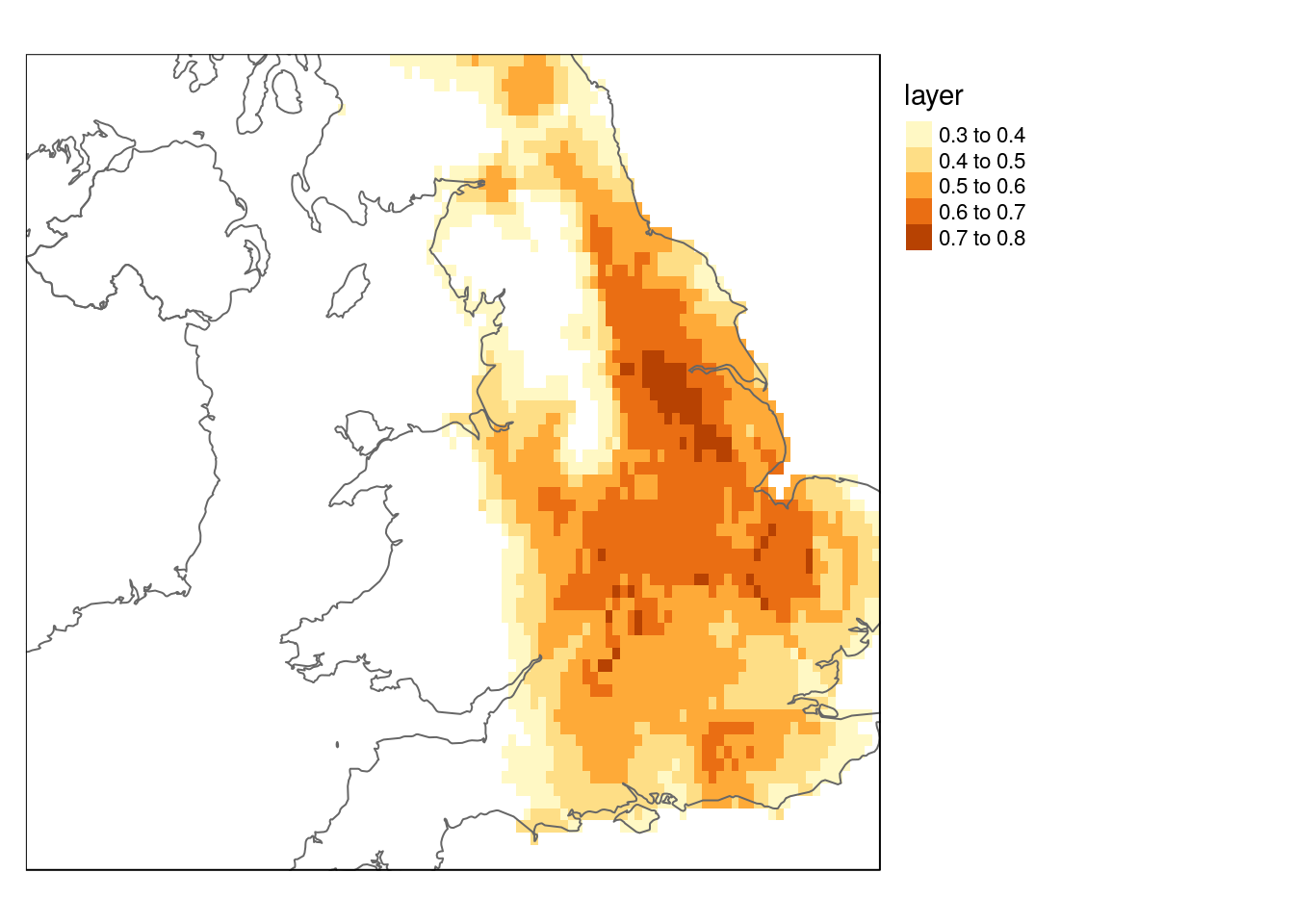
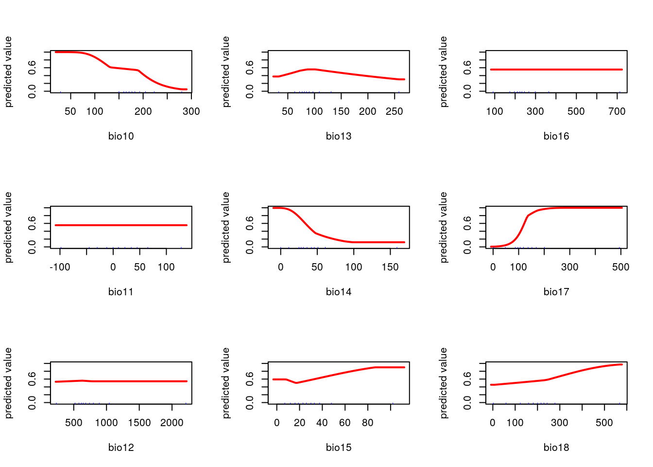
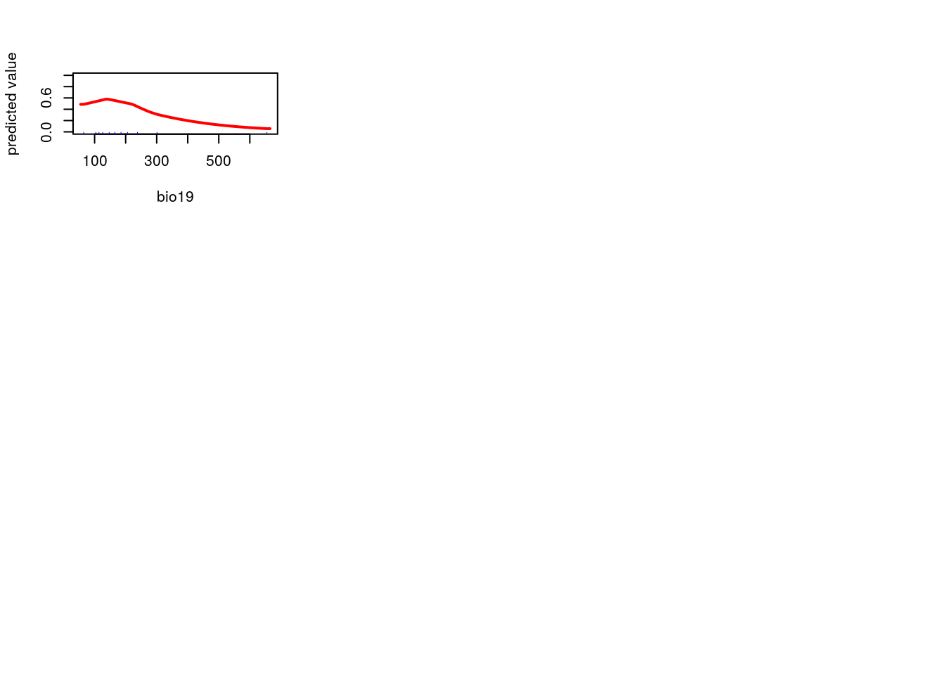
par(mfcol=c(3,3))
f<-function(x="bio1")response(me, var=x)
dd<-lapply(names(worldclim),f)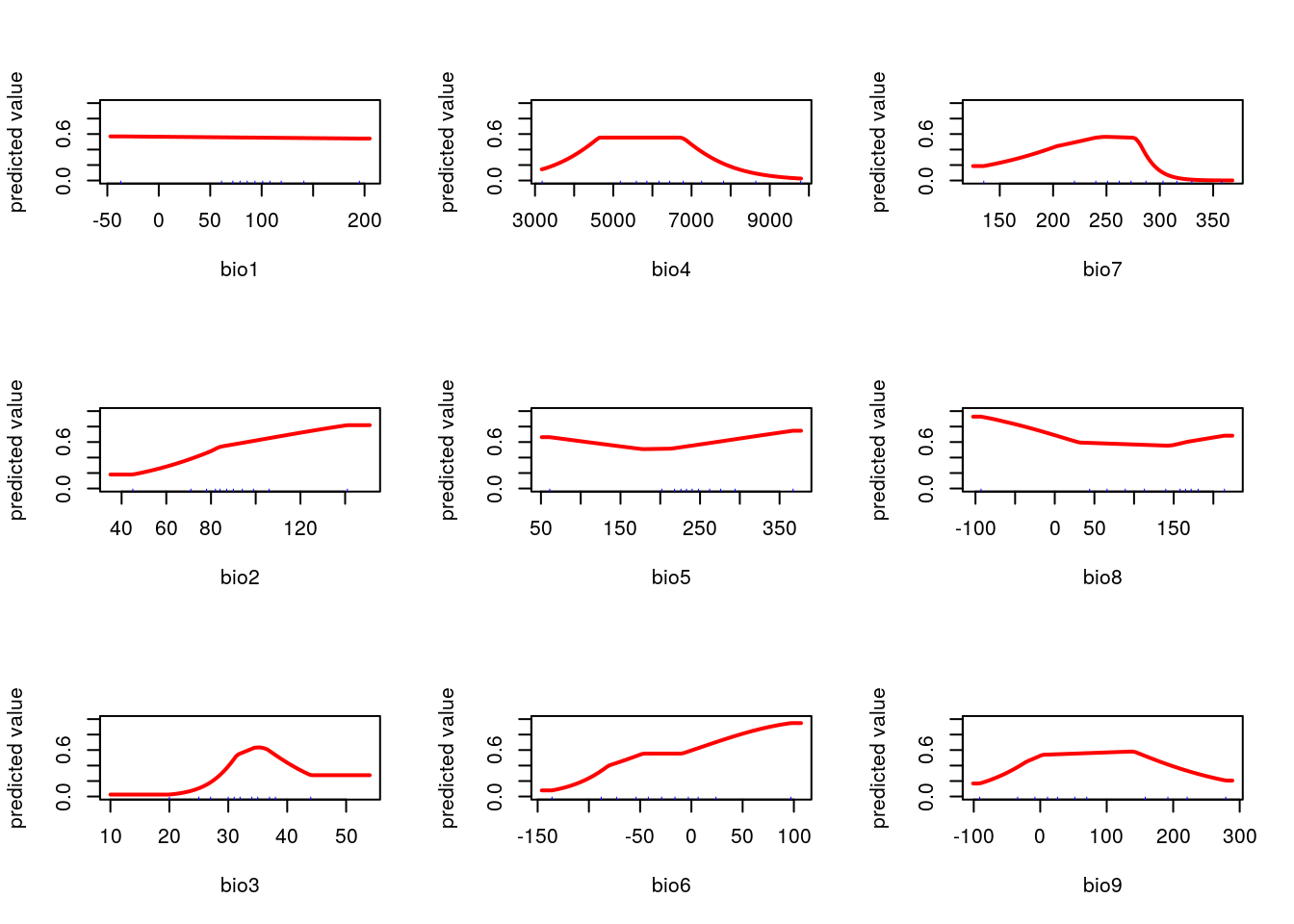
vetch<-st_read(conn,query="select * from gbif where
genus = 'Hippocrepis'")
vetch$an_temp<-raster::extract(worldclim$bio5,vetch)
unique(vetch$country)
#> [1] "France" "Spain"
#> [3] "Germany" "Greece"
#> [5] "United Kingdom" "Luxembourg"
#> [7] "Netherlands" "Italy"
#> [9] "Switzerland" "Austria"
#> [11] "Montenegro" "Romania"
#> [13] "Slovenia" "Slovakia"
#> [15] "Belgium" "Ukraine"
#> [17] "Tunisia" "Croatia"
#> [19] "Hungary" "Sweden"
#> [21] "Andorra" "Jersey"
#> [23] "Bosnia and Herzegovina" "Denmark"
#> [25] "Bulgaria"
vetch %>% filter(country %in% c("France","United Kingdom","Spain")) %>%
ggplot(aes(x=country,y=an_temp)) +geom_boxplot()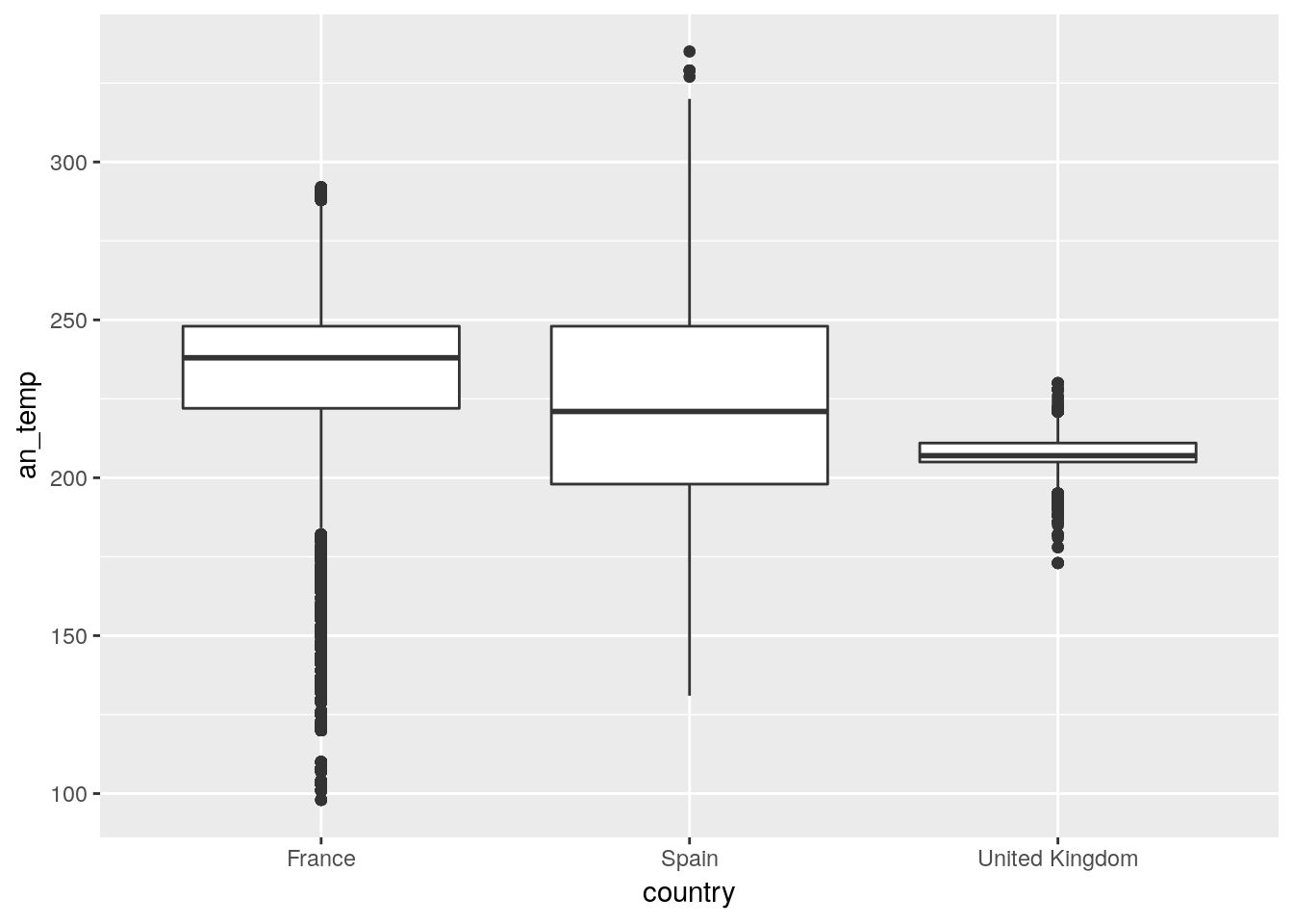
http://r.bournemouth.ac.uk:82/books/GIS_course/maxent/
dbDisconnect(conn)
rm(list=ls())
lapply(paste('package:',names(sessionInfo()$otherPkgs),sep=""),detach,character.only=TRUE,unload=TRUE)