Section 4 Spatial data bases
4.1 Concepts
Spatial data bases form the underlying core application of modern networked Geographical Information Systems. A spatial data base is like other networked data bases in many respects. Networked data bases are centralised, single point of entry, systems for information. For example, when you log on to conduct online banking you are using a networked database. In this case the data base must be provided with a huge number of secure features to prevent data from being accessed or altered by others. Spatial data bases use the same underlying technology. Data is held in a shared repository that can be updated in real time and can also be securely protected. For example, a company might use a spatial data base connected to web enabled GPS to track the position of delivery vans in real time.
The key advantage of a networked data base is data sharing. In the context of GIS analysis this means that the results of useful, and sometimes time consuming, work on spatial data can be easily provided to other users. It also means that everyone working on spatial tasks are looking at the same data at the same time. This improves comunication of methods and reproducibility of tasks.
Spatial databases can potentially contain very large amounts of information. It is therefore possible to run very large and complex operations over a large data set. However, when access to a database platform is being shared by many users at once this ability is usually restricted to a few superusers. Client applications of the data base are “served” data to prevent heavy usage crashing the system. So a spatial data base usually is linked to an application such as mapserver or geoserver which in turn will be used for producing web maps for users. See section 14. For example a geoserver can serve up all the priority habitats in the South of England as pictures within a web map. However this amount of data cannot be analyses in a visual context in its entirety. A sub set needs to chosen for analyses.
4.1.0.0.1 WMS visualisation of all priority habitats and SSSIs in South of England
This uses the geoserver and some R wrapper functions. See section ..
library(giscourse)

conn <- connect()
qmap("Dorset") %>% uk_wms() dbDisconnect(conn)
#> [1] TRUEThis map demonstrates why a data base is useful. Notice that although all the prority habitats can be visualised, the geoserver changes the resolution to meet the zoom level. This avoids forcing the software to try to render invisible geometries between vector points closer than the screen resolution. All the data behind the visualisation is not being used. One of the tasks of a spatial data base is to hold this information and provide access to subsets of it for analysis.
The data base for this course has been set up from large shapefiles and other sources using the code shown in the appendix Section 18
4.1.1 Data base work flow
If you are new to GIS or have only previously worked on a desktop GIS the concepts of using a shared data base may be unfamiliar. What does it mean to “connect” to a data base? Where is the information? How do tables in the data base tun into maps? How do I store my own work on a data base?
This course aims to answer most of these questions through practical examples. The key concept is that when you as a user are connected to a data base the information contained on a single centralised data server is accessible. The client application could be QGIS, R, ArcGIS or some other software. Each client has its own way of processing data. Once the data has been moved into the client environment it becomes like any other data in the client. So after loading a table from postgis into QGIS or ArcGIS it can then be treated as the equivalent of a shapefile, or data loaded in any other file format. However it is also possible to conduct operations directly on the data stored on the server. In this case it is the centralised server doing the work. Most users only are granted read access to shared data. So they can’t change the data. Think of a data base such as the Web of Science as an example. You can search and filter articles held on the data base in order to find information but you can’t alter anything. A spatial data base extends this concept, as some operations such as geoprocessing, spatial filtering and calculating statistics can also be implemented as operations on the server. After connecting to a spatial data base there are two ways of achieving the same results. Server side processing and client side processing. In most cases server side processing is only used briefly. It tends to be an intitial step used for subsetting data. This is rather like searching the Web of Science for a set of article that are then imported into Endnote or Mendeley for further analysis.
4.1.2 The sf package in R
The development of the sf package, that first became available on CRAN in 2015, made working with R and postgis quite seamless and interlinked. This is because the sf package and the postgis data base both use the same underlying formal data structure. A detailed technical explanation of this is provided here.
https://cran.r-project.org/web/packages/sf/vignettes/sf1.html
This vignette is very well written and provides a very useful reference, although some of the information is rather advanced at this stage.
Robin Lovelace’s book also has a useful section.
https://geocompr.robinlovelace.net/spatial-class.html#intro-sf
One of the nicest features of the sf package is the fact that function names used for client side operations within R match the names used in server side SQL. So R and postgis can be used together in quite a seamless manner which blurs the edges between server and client slightly. Operations involving the raw data stored as large tables on the server can be performed using SQL. Operations involving local subsets of the data are performed within R.
4.2 QGIS:Connecting to postgis
Connecting to the data base in QGIS involves the following steps.
- Click the postgis symbol on the browser panel (Elephant icon)
- Right click to open the dialogue for a new connection.
- Fill in the information needed.
- The name of the connection can anything you want. This is just to remind you what it is for.
- The host address is very important. It has to be typed correctly. At BU postgis is currently running on the address 172.16.49.31
- The server port is 25432 (not the default, which is 5432)
- The data base is named “gis_course”. Note the underscore.
These steps are shown in 4.1
Figure 4.1: Opening a connection to the postgis server: Adding the connection information. Host = 172.16.49.31, port =25432, database = gis_course
4.2.1 Providing username and password
The next step in the process of connecting is to provide a user name and password. The interesting element here is that data held on a spatial data base can be either shared with all users or held as private data. So if a data source is licensed to just a single user it can still be placed on the data base in a secure manner.
For the purposes of this course we are using publicly available data. Check the sources shown in 18 and make sure that you have registered as a user with the appropriate open data providers.
Action
- The authentication entry fields are found on the “basic” tab on the connection menu
- Add the user name gis_course
- The password for access to the public schema is gis_course123
- Click on test connection. You should see a blue message if the connection is successful.
- Click OK
- The connection now shows up on the browser tab. Clicking it will show the available vector layers in the data base.
The steps are shown in figure 4.2
Figure 4.2: Connecting step 2: Provide the username gis_course and password gis_course123: Click test connection
4.2.2 Connecting and adding layers
Now that the connection is made you can load data from the data base into your desktop project.
Please be careful Some of the layers are large. It is best not to load them directly by dragging them onto the canvas unless the map has been set to a local area. If in any doubt check the properties of the layers first. This is explained later.
Action
Load a light weight layer
- Find the layer named natural_earth_countries
- Click on the layer, or drag the layer onto the canvas
- You will see the layer added to the project.
This is shown in figure 4.3
Figure 4.3: Load the light weight natural earth countries layer by dragging it onto the canvas. PLEASE DO NOT DO THIS WITH THE LARGER LAYERS
In section 7 you will see how to subset large data sources for use in a project.
4.2.3 Inspecting the tables
The browser panel provides quick and simple access to all the vector tables held in the data base. However for more serious work you need to open the data base manager in QGIS. This is a very powerful tool which allows you to browse all aspects of the data held in the postgis data base that you are connected to without loading the data into the project canvas.
The most powerful feature of the data base manager is the ability to run spatially explicit sql queries. We will see how this works in later sections.
Action
- Open DB manager by clicking on the database tab on the top bar of QGIS
- Choose DM manager
- Select the postgis data base connection that you have already made.
- Browse the tables. You can see a list of all the columns in each table and their data types.
- Data can be previewed as both tables and maps. The caveat with this feature is that it should be used carefully with very large data sets.
Figure 4.4 shows these steps.
Figure 4.4: Using the data base manager in QGIS to inspect tables
Figure 4.5 shows the preview functionality in the data base manager.
Figure 4.5: Using the data base manager in QGIS to inspect tables
4.2.4 Structure of the tables
Notice that the tables of vector data held in the data base consist of columns of data, often called attributes in gis, plus one extra column that contains the geometry. This is the simple feature format. It may not seem that “simple”, but it is much more consistent than the old fashioned shapefile format. Shapefiles were a mess, as the essential data was split accross several files. The simple format is much more consistent and elegant. Once data is moved into QGIS it can be exported in any of the old or new GIS formats for use by users of other software.
4.3 RStudio:Connecting to the data base
As we saw in section 2.3.2 it is now very easy to produce web maps in R.
However R is a less visual environment when compared to QGIS. So when investigating the contents of a database it is often useful to use R in combination with the QGIS data base manager. Having the two program open together allows queries to be prototyped and tested in the QGIS db manager and then cut and pasted into an R script.
To connect to the data base in R we can use the RPostgreSQL package (there are other options such RODBC). A connection is established silently as an R object
A set of libraries are also typically needed to turn R into a GIS. So the code below would typically be included at the beginning of an analysis.
## Libraries
require(RPostgreSQL)
require(rpostgis)
require(sf)
require(mapview)
require(tmap)
## Connect
conn <- dbConnect("PostgreSQL", host = "postgis",
dbname = "gis_course" ,user = "gis_course", password = "gis_course123")After using the data base in R it is important to disconnect as keeping connections open may block other users.
## Disconnect
dbDisconnect(conn)
#> [1] TRUETo reduce typing all this has been rolled into a quick to remember function that checks the libraries and connects.
library(giscourse)
conn<-connect()
disconnect()
#> [1] TRUE
With a connection established tables from the data base can be loaded into R memory and visualised. However all the caveats that were mentioned with regard to rendering large layers in QGIS apply, and more so if mapview is being used.
To find a list of the tables in the data base from R directly.
conn<-connect()
dbListTables(conn) %>% as.data.frame() %>% DT::datatable()dbTableInfo(conn,"ph_v2_1") %>% as.data.frame() %>% DT::datatable()To get a simpler list of the attributes in a table
dbListFields(conn,"ph_v2_1")
#>  [1] "gid"        "objectid"   "main_habit" "confidence" "source1"
#>  [6] "s1date"     "s1habclass" "s1habtype"  "source2"    "s2date"
#> [11] "s2habclass" "s2habtype"  "source3"    "s3date"     "s3habclass"
#> [16] "s3habtype"  "base_mappi" "annex_1"    "additional" "candidates"
#> [21] "rule_decis" "general_co" "lastmoddat" "modreason"  "area_ha"
#> [26] "urn"        "shape_leng" "shape_area" "geom"
This is all useful to know if you are designing an analysis around priority habitats. Even so, it could have been quicker to just look at the table in QGIS. This is why using the two approaches to GIS “in tandem” is often a good approach.
A simple trick that can be very useful when designing queries on categorical attributes is to list all the possible values in a field. This is easier in R than trying to “eyeball” values in a table. See section 6
dbGetQuery(conn,"select distinct main_habit from ph_v2_1") %>% as.data.frame() %>% DT::datatable()The usefulness of this will become clearer in section 6
4.3.1 Using the sf package
The sf package provides most of the tools needed for communicating seamlessly with the spatial data base. Reading a table into R is simply a case of writing st_read(conn,“table_name”). The connection that is established at the start of the R session sends the request for the table to postgis and you can assign it an object name in R and begin working on it. However …
An example is shown in the code chunk below which produces figure 4.6
require(tmap)
countries<-st_read(conn,"nat_earth_countries")
qtm(countries)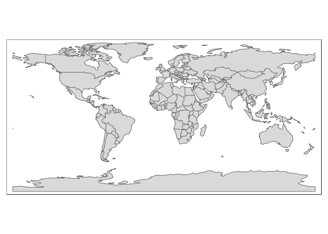
Figure 4.6: The nat_earth_countries table loaded into R and visualised using the quick map function from tmap.
4.3.2 Loading only geometries
Postgis is a spatial extension to the postgresql data base. Not all the tables held in the data base need to be spatial. The data base can be used more generally to hold other forms of data, that may be linked to spatial data when needed. For example data concerning counties, countries, administrative districts etc can all be held in no spatial format in postgresql. Providing they also have some field that occurs in a spatial table they can be linked to the geometry and mapped out as required.
If we just want to get the geometry from a postgis table we need to know the name that is used for the geometry column. This is not always consistent, as there are different default settings used when loading data into the data base. In the past the geometry column was ofthen named “the_geom”. However this is now deprecated. In the gis_course data base all geoetries are called either “geom” or “geometry” depending on whether they were loaded directly from R or by gdal.
We can try a very simple query to return just the geometry. A safe option for potentially large tables is to just get a few geometries to look at by using a limit. So any of these queries will produce a quick map if run. Setting a limit is a good safe way of eyballing a geometry just to see what it looks like. You can also load it in to check the coordinate reference system.
# Not run here
st_read(conn, query ="select geometry from gbif limit 10") %>% qtm()
st_read(conn, query ="select geom from counties limit 10") %>% qtm()
st_read(conn, query ="select geometry from waterways limit 10") %>% qtm()
All the tables in the gis_course data base have been loaded using either gdal or R with default settings. Those loaded with st_write from R have a geometry table named geometry. The rest have geometry tables named geom. So if a query returns an error with one name, change to the other and it will work. The only exception to this are the open street map layers. The names “way” is used to describe the geometries in these layers, which also require special handling.
4.3.3 Disconnect from the data base
Always run this at the end of any session.
dbDisconnect(conn)
#> [1] TRUE
## or simply disconnect() using giscourse library