Section 12 Map algebra
12.1 Concepts
The term map algebra typically refers to operations conducted on multiple raster layers using mathematical expressions and boolean logic. It can be used to build up the complex algorithms used by hydrologists and geomorphologists. Map algebra is also frequently used by ecologists and geographers to build up bespoke calculations of indices that combine many layers, such as human impact, habitat suitability etc.
12.2 Map algebra in R
The development of the r raster package by Robert Hijmans revolutionised the way raster data is handled in R. The raster package makes map algebra simple, intuitive and elegant. So much so that there is little point in showing any alternative methods in an introductory course, as they are all much more difficult to learn. The only caveat with regards to using the raster package is that although it will handle most jobs it is not well suited to the very largest raster layers. In these cases GRASS remains one of the best open source options for handling operations on extremely large rasters. Postgis can also be used for huge multitemporal raster processing, but this is quite complex and won’t be shown on this course.
12.2.1 Getting Worldclim layers
require(mapview)
require(leaflet.extras)
library(tmap)
require(raster)
require(rgdal)

mapviewOptions(basemaps =c("OpenStreetMap","Esri.WorldStreetMap", "Esri.WorldImagery", "CartoDB.Positron", "OpenTopoMap", "OpenStreetMap.BlackAndWhite", "OpenStreetMap.HOT","Stamen.TonerLite", "CartoDB.DarkMatter", "Esri.WorldShadedRelief", "Stamen.Terrain"))
In addition to providing a simple to use platform for processing raster layers, the raster package (and the dismo package) provide easy access to data sets held on the cloud. The worldclim data set is very commonly used for analysing global climate patterns and is particulary widely used in species distribution modelling.
The raster package has an extremely handy and well designed “get_data” function. Not only does this function pull down raster tiles using very inutuitve options to alter the extent and resolution, the function sensibly stores the results locally so that if the file has already been downloaded it is not fetched from the internet again.
The lines below build raster bricks for precipitation, minimum temperature, maximum temperature, elevation (altitude)
## Set a low resolution for demo purposes.
library(raster)
path<- "~/geoserver/data_dir/rasters/worldclim"
res<-10
worldclim_prec<-getData(name = "worldclim", var = "prec", res = res,path=path)
worldclim_tmin<-getData(name = "worldclim", var = "tmin", res = res,path = path)
worldclim_tmax<-getData(name = "worldclim", var = "tmax", res = res,path=path)
worldclim_bio<-getData(name = "worldclim", var = "bio", res = res,path=path)
worldclim_alt<-getData(name = "worldclim", var = "alt", res = res,path=path)
12.2.1.1 The world altitude layer
We can reuse some code from the terrain analysis section to quickly visualise world elevation at this scale. This only really makes sense for the highest mountains, so the map is centred around the Himalayas.
wslope<-terrain(worldclim_alt, opt='slope', unit='radians')
waspect<-terrain(worldclim_alt, opt='aspect',unit='radians')
whill<-hillShade(wslope,waspect,angle=5)

plot(whill, col = gray(0:100 / 100), legend = FALSE, xlim=c(40, 120), ylim=c(10, 60))
plot(worldclim_alt, col = terrain.colors(25), alpha = 0.4, legend = TRUE, add = TRUE, xlim=c(40, 120), ylim=c(10, 60))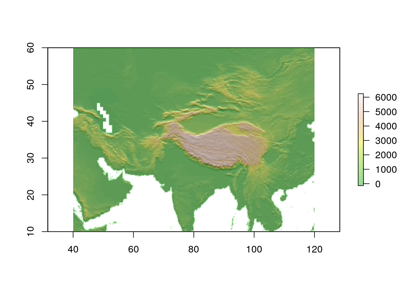
12.2.1.2 SRTM data for the UK
The raster package also provides an easy way to download and use the shuttle radar telemetry (SRTM) global elevavation layer at 90m resolution. As this coverage has a high resolution at the global extent, the layer is downloaded as tiles. The functon takes a coordinate falling within the tile as input. There are five tiles for the whole of the UK and the Island of Ireland.
path<- "~/geoserver/data_dir/rasters/srtm"
srtm1<-getData('SRTM', lon=-2, lat=55,path=path)
srtm2<-getData('SRTM', lon=1, lat=55,path = path)
srtm3<-getData('SRTM', lon=-6, lat=55, path= path)
srtm4<-getData('SRTM', lon=-2, lat=60, path = path)
srtm5<-getData('SRTM', lon=-6, lat=60, path = path)
The raster package has a useful merge function that joins up the tiles into a continuous tif file. So we can make one like this.
# srtm<-merge(srtm1,srtm2,srtm3,srtm4,srtm5)
# writeRaster(srtm,file="rasters/srtm_uk.tif")
This is a bit slow and the same effective result is also achieved by using a vrt (see next section)
path<- "~/geoserver/data_dir/rasters/srtm"
system(sprintf("gdalbuildvrt rasters/srtm.vrt %s/*.tif",path))
Now loading the raster layer from a file is very simple. Just use the raster function to assign it to an object in R. Notice that this is a “lazy” evaluation that does not load the raster into memory. The raster declaration simply makes a reference to it.
Always check on the size of the raster before going any further.
# Either
srtm<-raster("rasters/srtm_uk.tif")
# Or
srtm<-raster("rasters/srtm.vrt")
dim(srtm)
#> [1] 12001 18001     1
The product of the dimensions divided by 1000000 gives the size in MB
prod(dim(srtm))/1000000
#> [1] 216.03
This (i.e 216 MB) is a manageable file. size in R. However the actual data is still on disk. There will only be issues with memory if we carry out operations such as trying to place it all into a single mapview.
12.2.1.3 Cropping a raster layer in R
Cropping raster layers results in a smaller extent and so lighter demands on memory. The easy way to do this is to use a polygon to set the bounds. Notice that this does not remove pixels falling outside the polygon itself. It crops to the bounding box.
We’ll get a polygon for Dorset from the natural earth layer. We don’t need to connect to the data base for any of this part.
library(rnaturalearth)
library(dplyr)

counties<-ne_states(country = 'United Kingdom', returnclass = c("sf"))
counties %>% filter (name=='Dorset') %>% as("Spatial")->dorset
dorset_srtm<- raster::crop(srtm,dorset)

dslope<-terrain(dorset_srtm, opt='slope', unit='radians')
daspect<-terrain(dorset_srtm, opt='aspect',unit='radians')
dhill<-hillShade(dslope,daspect,angle=5)

plot(dhill, col = gray(0:100 / 100), legend = FALSE)
plot(dorset_srtm, col = terrain.colors(25), alpha = 0.4, legend = TRUE, add = TRUE)
plot(dorset,add=TRUE)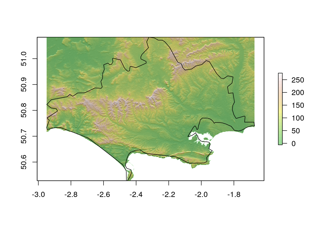
Let’s have a look at this with a mapview.
library(RColorBrewer)
pal1<-terrain.colors(100)
pal2<-gray(0:100 / 100)
pal1 <- colorRampPalette(pal1)
pal2 <- colorRampPalette(pal2)

map<-mapview(dorset_srtm,col.regions=pal1, legend=FALSE) + mapview(dhill,col.regions=pal2, legend=FALSE)
map
If we did really want to just work on the SRTM for Dorset we use the mask function to cover areas that are not in Dorset. Any analysis after a mask only uses those pixels.
masked_dorset_srtm<-mask(dorset_srtm,dorset)
plot(masked_dorset_srtm)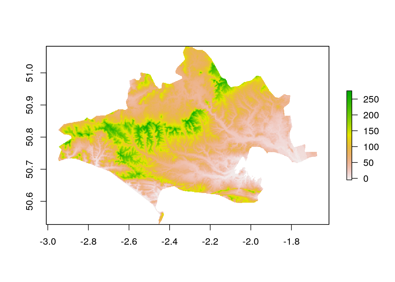
12.2.2 Raster statistics
The nice part of doing GIS in R is that all the familiar statistical functions are at hand, so any question that you want to ask of the data is just a line of code away. Raster layers are treated just like any other matrix, so we can ask for a summary.
summary(masked_dorset_srtm)
#>           srtm
#> Min.        -5
#> 1st Qu.     47
#> Median      78
#> 3rd Qu.    117
#> Max.       276
#> NA's    552569
So the median elevation of the county is 78 meters and the highest point is at 276 meters. Let’s find the highlands of Dorset which we’ll define as land over 100 meters. This is a simple one liner in R.
contours<-rasterToContour(masked_dorset_srtm,levels=c(100))
plot(masked_dorset_srtm>100)
plot(contours, add= TRUE)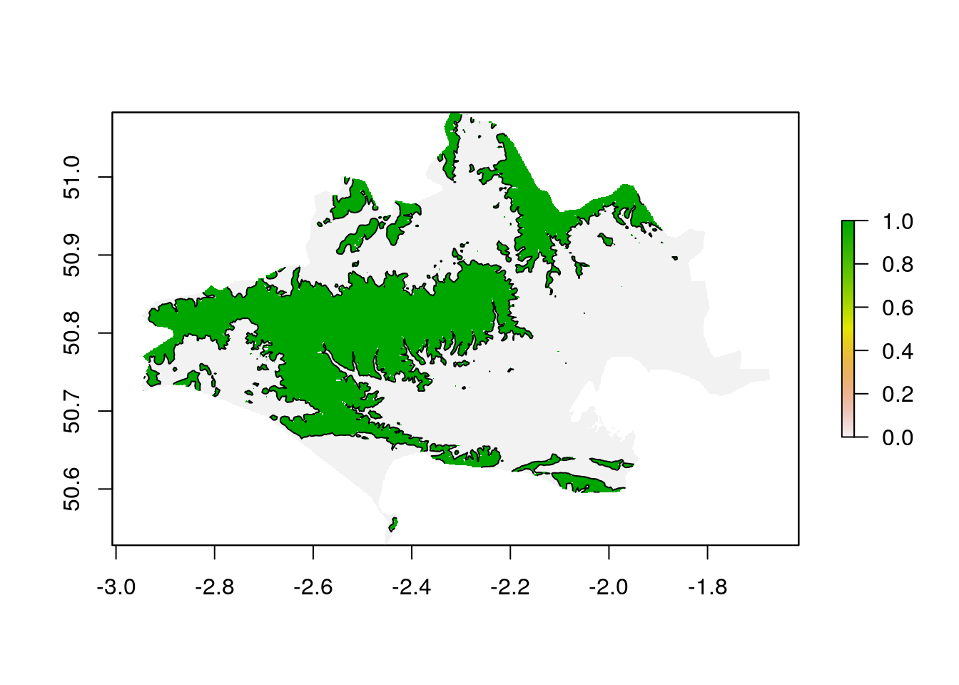
If we want to know what proportion of Dorset is over 100m we need to know the number of pixels in dorset and the number of pixels over 100m
vals<-na.omit(getValues(masked_dorset_srtm)) ## Just take the non masked values

sum(vals>100)/sum(vals>0)
#> [1] 0.3432775
So 34% of the land surface of Dorset lies over 100m above sea leval.
Let’s try something a little bit harder. Find all the steep(ish) south facing slopes.
We’ll use these definitions.
Steep = slope greater than 5 degrees South facing = aspect between 130 degrees and 230 degrees
This is a boolean operation.
## Get terrain
slope<-terrain(masked_dorset_srtm, opt='slope', unit='degrees')
aspect<-terrain(masked_dorset_srtm, opt='aspect', unit='degrees')

## Find slopes and set rest to NA
steep_south_slope<-(slope>5 & aspect> 130 & aspect< 230)
steep_south_slope[steep_south_slope<1]<-NA


map + mapview(steep_south_slope,legend=FALSE, na.color ='transparent')
Providing layers are of the same extent and the same resolution any sort of mathematical operation can be performed on them together. It is as simple as writing a formula in R to combine a set of vectors.
12.2.3 Multiple rasters held in a stack (or brick)
A great feature of Hijmans raster package is the use of raster stacks and/or bricks. The idea is similar to a multiband raster, but the elements of a stack or brick can be in separate files. They all must have the same resolution and extent.
class (worldclim_prec)
#> [1] "RasterStack"
#> attr(,"package")
#> [1] "raster"
The worldclim precipitation object is a raster stack. Raster bricks work in the same way as stacks, but processing a brick can sometimes be wuicker as they are forced into memory. It is usually safer to work with stacks. You can find the dimenstions with dim.
dim(worldclim_prec)
#> [1]  900 2160   12
Notice that there are three dimenstions. The third is the number of layers, which in the worldclim case is 12, i.e. one for each month of the year. A default print of the stack produces 12 maps.
plot(worldclim_prec)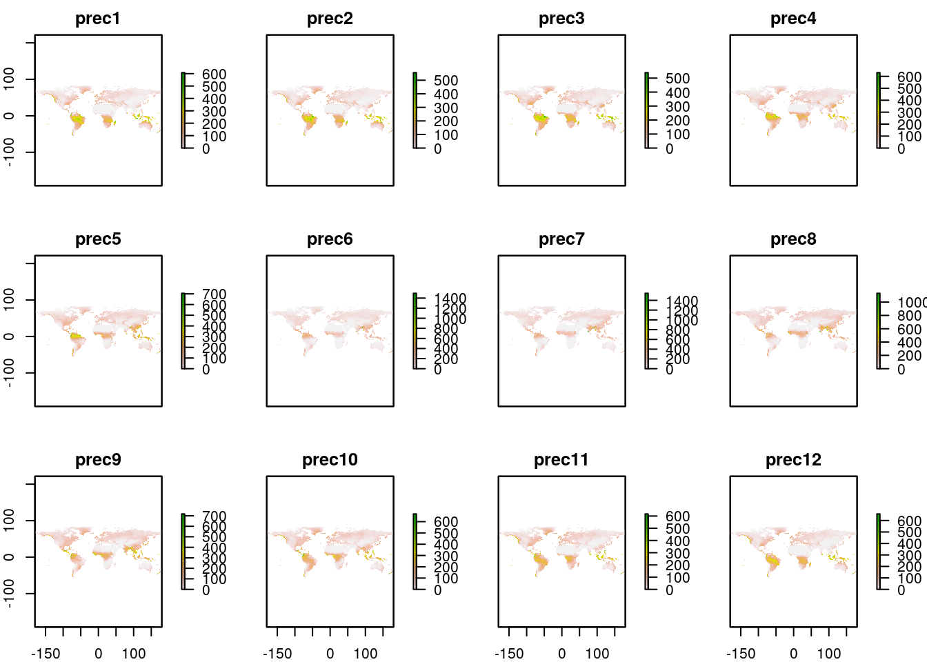
The neat feature is that functions work on the stack by driling through the 12 layers. To understand this, let’s get a map of total annual rainfall. This is really easy,
anprec<-sum(worldclim_prec)require(RColorBrewer)
pal <- colorRampPalette(brewer.pal(9, "BrBG"))
mapview(anprec, col.regions = pal(100), at = c(0, 100, 300,600,1000,3000,10000), legend = TRUE)12.2.4 Calculating the mean monthly temperature
Two stacks with the same number of layers can also be combined in a really simple way. So a rough mean monthly temperature can be found by adding the maximum and minimum and dividing by 2. The original Worldclim layers hold temperatures as integer values (i.e. the actual value rounded ot one decimal point and multiplied by 10) in orer to save space. When the mean is taken a floating point will result, so at this point we may as well divide by 20 rather than 2 to get the result in degrees centigrade.
worldclim_tmean<-(worldclim_tmax + worldclim_tmin) / 20
plot(worldclim_tmean)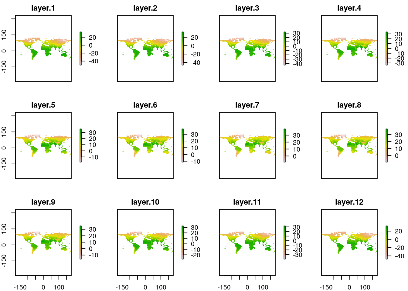
This is all very neat. It almost looks as if the raster package was designed to make working with worldclim data easy. I wonder why that might be?
So, mean annual temperature can now be found
an_mean_temp<-mean(worldclim_tmean)require(RColorBrewer)
pal <- colorRampPalette(brewer.pal(9, "RdBu")[9:1])
mapview(an_mean_temp, col.regions = pal(100), at = c(-40, 0, 5,10,15,20,25,30), legend = TRUE)12.3 Exercise
The bioclim layers have all been derived from the Worlclim tmax, tmin and prec layers with map algebra. How many of them can you derive?
BIO1 = Annual Mean Temperature
BIO2 = Mean Diurnal Range (Mean of monthly (max temp - min temp))
BIO3 = Isothermality (BIO2/BIO7) (* 100)
BIO4 = Temperature Seasonality (standard deviation *100)
BIO5 = Max Temperature of Warmest Month
BIO6 = Min Temperature of Coldest Month
BIO7 = Temperature Annual Range (BIO5-BIO6)
BIO8 = Mean Temperature of Wettest Quarter
BIO9 = Mean Temperature of Driest Quarter
BIO10 = Mean Temperature of Warmest Quarter
BIO11 = Mean Temperature of Coldest Quarter
BIO12 = Annual Precipitation
BIO13 = Precipitation of Wettest Month
BIO14 = Precipitation of Driest Month
BIO15 = Precipitation Seasonality (Coefficient of Variation)
BIO16 = Precipitation of Wettest Quarter
BIO17 = Precipitation of Driest Quarter
BIO18 = Precipitation of Warmest Quarter
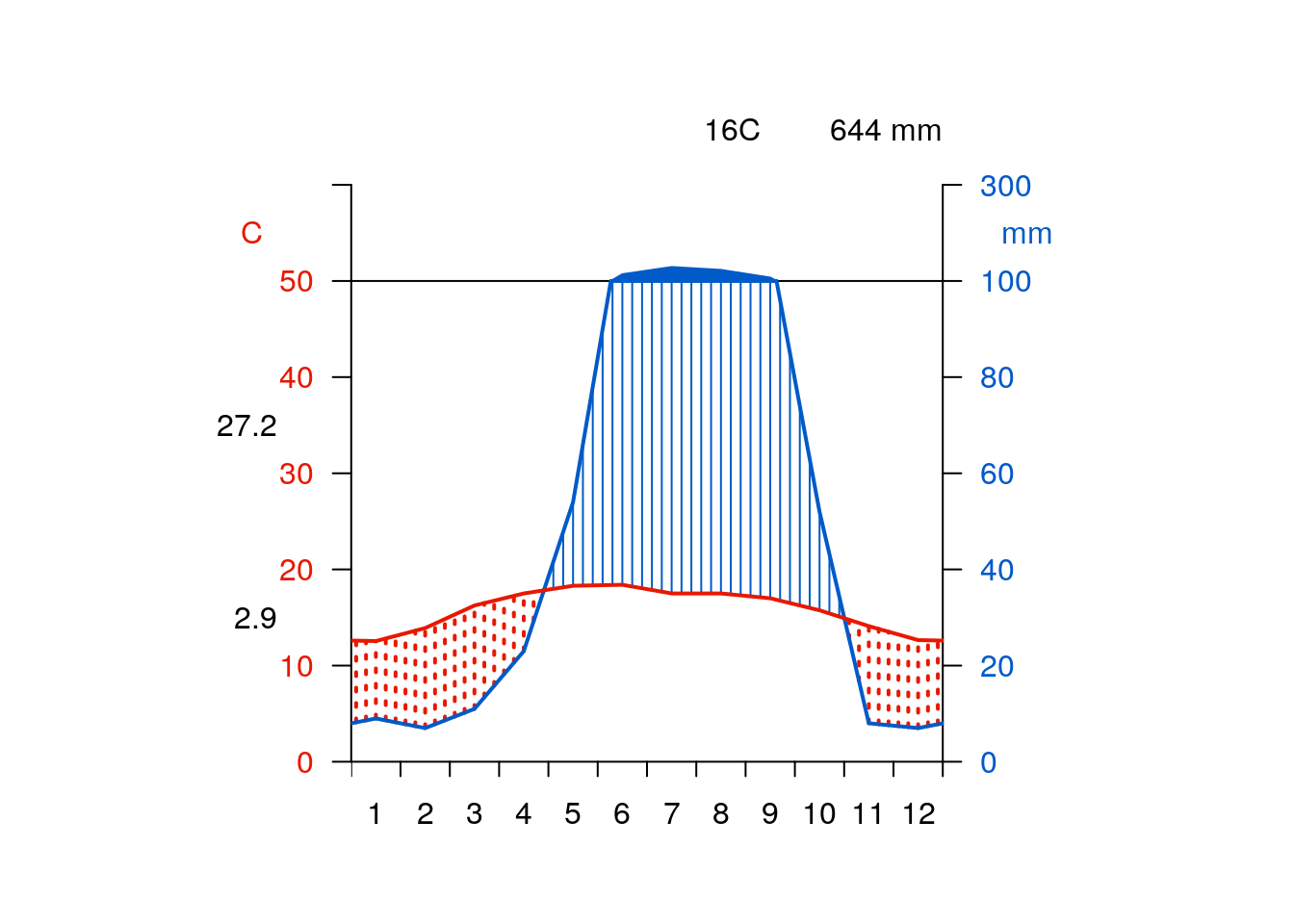
BIO19 = Precipitation of Coldest Quarter 12.4 Extra bonus: Making climate diagrams for anywhere in the World
One of the motivations behind the worldclim data set is its use in species distribution modelling. The raster extract function adds climate data to any coordinates from WorldClim. So we can add a little utility function to the giscourse package very easily that combines geocoding with Worldclim as a quick look up.
getwclim<-function(place="Bournemouth",res=2.5) {
path<- "~/geoserver/data_dir/rasters/worldclim"
prec<-getData(name = "worldclim", var = "prec", res = res,path=path)
tmin<-getData(name = "worldclim", var = "tmin", res = res,path = path)
tmax<-getData(name = "worldclim", var = "tmax", res = res,path=path)

require(tmaptools)
pnt<-as(geocode_OSM(place,as.sf=TRUE),"Spatial")
tmins<-unlist(raster::extract(tmin,pnt)/10)
tmaxs<-unlist(raster::extract(tmax,pnt)/10)
precs<-raster::extract(prec,pnt)
df<-data.frame(prec= as.vector(precs),tmax = as.vector(tmaxs),tmin=as.vector(tmins))
df
}

getwclim()wldiag<-function(df){
require(climatol)
mat<-rbind(df$prec,df$tmax,df$tmin,df$tmin)
diagwl(mat)
}require(giscourse)
place<-"Bala, Wales"
qmap(place)getwclim(place) %>% giscourse::wldiag()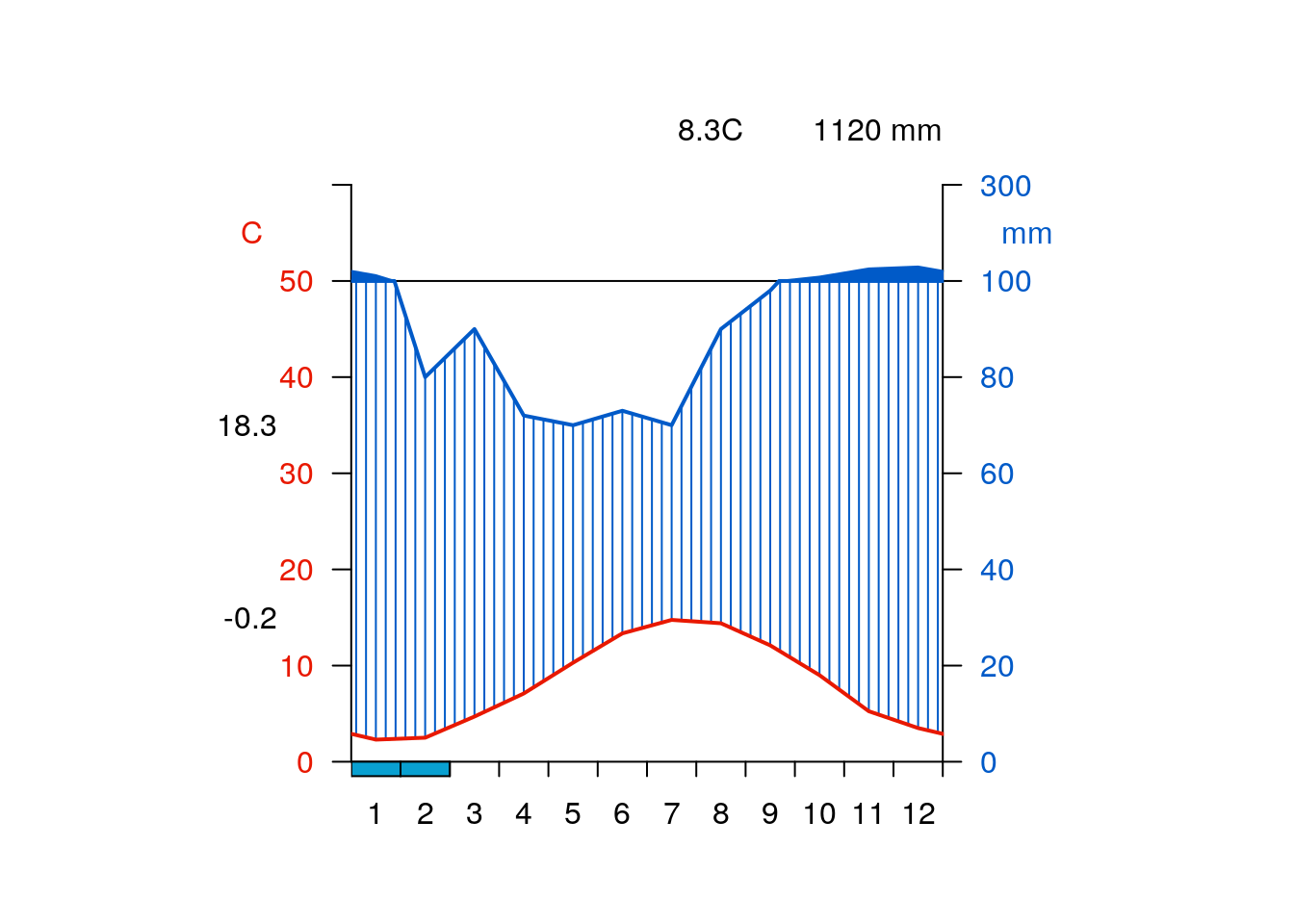
place<-"Mexico city"
qmap(place)getwclim(place) %>% giscourse::wldiag()