Section 8 Making maps; Digitising and cartography

8.1 QGIS

8.1.1 Digitising in QGIS

This section needs updating. Meanwhile refer to old course handouts found here. Right click the links to open in a new tab, as the links takes you out of the current bookdown and into another.

Link to chapter on digitising

8.1.2 Cartography in QGIS

Link to chapter on styling

8.2 R: Map making

require(tmap)
require(mapview)
require(giscourse)
conn<-connect()

8.2.1 Web maps in R

Forming zoomable slippy web maps in R has been possible for many years. However it has recently become trivially simple to obtain webmaps after the addition of the mapview package. Mapview is a high level wrapper to the leaflet package which is in turn an R wrapper around leaflet maps in java. This means that it is possible to alter many aspects of the default web maps produced by mapview by making alterations at a lower level. However the great advantage of mapview is the ease of use. This means that web maps can be quickly produced while programming an analysis in order to check results. These quick views do not necessarily appear in a final analysis. They make working in R much more like working directly in a more visual environment such as QGIS. This changes the workflow. It reduces the need to to use a GUI based GIS alongside R. It makes it simpler to work on the code of an analysis and check the results as you go.

8.2.2 Saving web maps

There are several ways of saving the maps you produce in R and pass them to others. The nice element of the leaflet package used by maptools is that the maps are fully self contained i.e. you don’t need R to see them nor do you need a connection to postgis to look at data that has been passed from postgis to R. An R webmap is simply a piece of HTML. So a document with maps can be saved and sent to others to look at and/or embedded in another web page. Mapview maps can also be assigned to an R object and saved as a binary file that can be used by another R user or passed from one analysis to the next. The simplest way to make a clean standalone web page is to place code in a clean markdown document. Remove headers and set echo set to false, so the code is not shown. Then knit and save the file.

8.2.3 Base maps

A list of base maps can be found here

One way to quickly set the base maps is to form a list of all those that may be useful then subset it.

base_maps<-c("Esri.WorldImagery","OpenStreetMap","Esri.WorldStreetMap", "CartoDB.Positron", "OpenTopoMap", "OpenStreetMap.BlackAndWhite", "OpenStreetMap.HOT","Stamen.TonerLite", "CartoDB.DarkMatter", "Esri.WorldShadedRelief", "Stamen.Terrain")

mapviewOptions(basemaps = base_maps[c(2,1)])

8.2.4 Geocoding

An extremely useful feature of R is the built in Geocoding. If you have a Google account the Geocoding can use that. However this is an open source course, so we will use open street map geocoding. This is very simple. Just type the place name into the function.

This produces a central coordinate and bounding box.

require(tmaptools)
geocode_OSM("Wareham")

## $query
## [1] "Wareham"
## 
## $coords
##         x         y 
## -2.109838 50.686897 
## 
## $bbox
##      xmin      ymin      xmax      ymax 
## -2.149838 50.646897 -2.069838 50.726897

Some place names need more details to ensure that the right match is found.

A small utility function using this is included in course package. With the package loaded just type qmap with the name of the place you want to pop up a web map. This can be piped into another utility function in the package that adds extra features including a geocoding search tool, a measuring tool and a collapsible overview map.

require(giscourse)
qmap("Arne, Dorset") %>% extras()

8.3 Drawing and saving your own features in R

R is not a suitable tool for serious digitising work. There would be no point in developing R packages for digitising, as QGIS is available for that. However there are times when it is convenient to capture a polygon or set of points in R while working on an analysis. This is easy

8.3.1 Example for points

Students sometimes forget to capture the position of their sites with gps and can only identify them on a map. The go to fix is to use Google maps. There is no need to leave R.

In this example we quickly georeference some points. The emap function is a little wrapper function to mapedit that is included in the course package. It will only run interactively. The screenshot figure 8.1 shows the way to use it. Just run the code, make the map full screen and digitise.

Capturing some points with emap. Just run the code chunk while working on an analysis. The default is to capture the points to the open postgis connection. If you don't want to do this, or you don't have a connection open include write=FALSE in the code. Notice that in RStudio the map appears in the plots window. You need to make it full screen by clicking zoom.

Figure 8.1: Capturing some points with emap. Just run the code chunk while working on an analysis. The default is to capture the points to the open postgis connection. If you don’t want to do this, or you don’t have a connection open include write=FALSE in the code. Notice that in RStudio the map appears in the plots window. You need to make it full screen by clicking zoom.

# sites<-emap(write=FALSE) if no connection open
#sites<-emap(table="mysites") # Writes to postgis.

Make sure you click the points in exactly the same order that you have the sites in the data frame you want to georeference.

To add the geometry to the attributes in your sites data frame you need to have a common column to merge on. The easiest fix is to make an id column on both the data frame and the geometry numbered from one to the length of the geometry.

nsites<-length(sites$geometry)
df<-data.frame(id=1:nsites,sites=paste("site",1:nsites,sep="_"))
sites$id<-1:nsites
sites<-merge(sites,df)

Now you have your sites with latitude and longitude points. To get X and Y in British National grid it’s simply st_transform.

st_coordinates(st_transform(sites,27700))

##          X        Y
## 1 396258.1 93934.14
## 2 397416.6 96691.23
## 3 401386.4 98536.65
## 4 405066.7 97949.47

The same approach can be taken with site outline polygons. The mapedit can return mixed geometries of points and polygons. These are not easy to handle, so you should just choose one type of object at a time.

This approach is only useful as a quick fix when working in R. The mapditor does not have any more sophisticated features such as snapping.

Lovelace’s book has many useful sections an advice on map making.

8.4 Printable maps in R

There are multiple ways of producing static, printable maps in R that have evolved over time.

The most recent, high level package to emerge is tmap. This greatly simplifies map making by setting sensible defaults. Themes can be changed to alter the style without changing other elements of the code.

There is a section on tmaps in Lovelace’s book link

There is also a very good getting started vignette on Tmaps. There is no point in repeating all the information here.

Getting started with tmaps
[]

8.4.1 Using qtm

The fastest possible way to make a map.

query<-"select mhabitat,st_buffer(st_union(geom),0.1) geom 
from arne.phabitat group by mhabitat "
habitat<-st_read(conn,query=query)

qtm(habitat, "mhabitat", palette = "RdYlGn") +tm_layout(legend.outside=TRUE)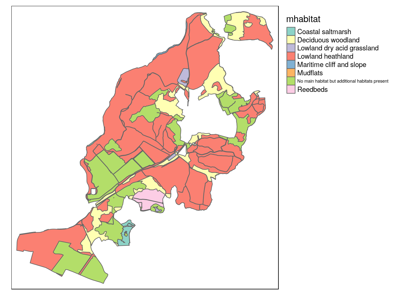

Figure 8.2: The hardest part of cartography is getting the palette right. This was a very poor choice.

8.4.2 Animated charts in R

If you have spatial data which forms a temporal sequence the leaflet minicharts package can turn the data into animated charts placed on the map. There are two types that are useful. Bubble plots which change in size and barcharts. The data base has a table of counts of blue butterflies on transects in Dorset.

require(leaflet.minicharts)

## Loading required package: leaflet.minicharts

counts<-st_read(conn,"blues_counts")
mapview(counts,zcol="species",burst=TRUE)

The minicharts are mapped onto leaflet maps using raw coordinates, unlike mapview which takes an sf object directly. So some data manipulation is needed. The format required is a data frame with columns for each variable (wide format), two columns for the latitude and longitude and one for the time.

counts %>% group_by(year,site) %>% summarise(adonis=sum(count[species=="pbellargus"]), chill=sum(count[species=="pcoridon"])) %>% filter(year>1989) ->counts2
data.frame(counts2[,1:4],st_coordinates(counts2)) ->counts2
str(counts2)

## 'data.frame':    498 obs. of  7 variables:
##  $ year    : int  1990 1990 1990 1990 1990 1990 1990 1990 1991 1991 ...
##  $ site    : chr  "ballard_down" "fontmell_down" "hod_hill" "magdalen_hill_down" ...
##  $ adonis  : int  181 655 131 0 14 0 0 0 128 116 ...
##  $ chill   : int  3 1281 58 437 226 799 268 1747 8 18 ...
##  $ geometry:sfc_POINT of length 498; first list element:  'XY' num  -1.97 50.63
##  $ X       : num  -1.97 -2.17 -2.21 -1.29 -1.41 ...
##  $ Y       : num  50.6 51 50.9 51.1 50.7 ...

Now set up a blank map.

mp<-mapview(counts)

8.4.3 Animated bubble charts

8.4.3.1 Adonis blue animated map

library(leaflet.minicharts)
mp@map %>%
  addMinicharts(
    counts2$X,counts2$Y, 
    chartdata = counts2$adonis,
    width=100,
    height=100,
    showLabels = TRUE,
    time = counts2$year
   
  )  %>% addFullscreenControl()

Figure 8.3: Adonis blue total annual counts over time. Note shown as screenshot as does not render in the bookdown format

8.4.4 Animated barcharts

mp@map %>%
  addMinicharts(
    counts2$X,counts2$Y, 
    chartdata = counts2[,3:4],
    time = counts2$year,
   width = 45, 
   height = 100)  %>% addFullscreenControl()

Figure 8.4: Adonis and chalkhill blue total annual counts over time

Introduction to open source GIS