Introduction to open source GIS
2019-05-29
Section 1 Introduction to the course
“Well, in our country,” said Alice, still panting a little, “you’d generally get to somewhere else if you run very fast for a long time, as we’ve been doing.” “A slow sort of country!” said the Queen. “Now, here, you see, it takes all the running you can do, to keep in the same place”
Open source GIS is a very fast moving field. The great thing about running fast in order to keep up with all the new developments in OS GIS is that you do in fact get to somewhere by doing so. The down side of working on a moving target is that any advice that you may give regarding the specifics of actually doing GIS is likely to be obsolescent the moment after it is provided. This makes writing course notes very challenging.
There is also no getting around the fact that doing GIS can be time consuming. The spatial data world is complex and a large number of concepts and skills need to be assimilated. Problem solving skills are essential. However the time spent on GIS analysis can be dramatically reduced by adopting good practice. The solution to one problem always provides the solution to another similar problem. This is the key to reproducible GIS. Writing down a solution to a problem in the form of a script solves all similar problems permanently. With experience GIS analysis becomes faster to implement through reapplying old techniques to new problems.
Modern GIS software provides access to an increasing number of algorithms and tools. It is natural to feel rather overwhelmed by the large number of options. The approach taken in this course has been to use the 80:20 rule. Although obtaining perfect results takes up 80% of your effort in any GIS project, getting started should only take 20% of the time but can still produce results that are 80% along the path. Both QGIS and R have improved out of recognition with respect to usability. Long time users of both QGIS and R may be unaware that there are now much easier ways to obtain results quickly than when they first started to use the software.
This course follows many of the same themes that are covered in the book that motivated the course. https://geocompr.robinlovelace.net/intro.html. Links to relevant chapters in the book have been added to this course material. There would be no point in duplicating all the information in Robin Lovelace’s excelent book. Instead I have aimed to make sure that all the techniques shown in that book can also be implemented by anyone with a log in to the BU server. Code from the geocompr book can be used to build more advanced analyses using the data provided here.
This course differs from the geocompr book through placing more emphasis on the use of a networked spatial data base on a server. The postgis spatial database forms a link between the R and QGIS though which data can be shared and transfered. Although the examples can be followed without access to the server, they will only run as shown when logged on to the BU system.
Most of the sections in the course consist of three parts. First the conceptual elements are briefly outlined These elements should be relatively immune from the Red Queen effect and are common to all GIS.
The rest of each section is typically split into two practical sub sections. The first shows how to use the concepts with open source desktop GIs (QGIS). This has a point and click interface. Animated gif screenshots are included to help demonstrate the steps, particulary at the beginning. The second part implements the same theory using R scripts. GUI interfaces may change. New R packages may emerge and evolve, so these sections may need updating continuously. However, this is the most reproducible element of the course. All the R code that is shown has been run through the server when this document is compiled. It produced all the maps and figures. Anyone with access to the BU server can run the same code again and they will see exactly the same output. Changing input data or options in the code will produce new results. The code forms a starting template to be adapted to produce new pieces of work.
This is an introductory course. Each section only scratches the surface of a theme. The examples have been chosen to be particularly relevant to Bournemouth students. All the steps shown in QGIS or in the R code can be adapted to other contexts. The central theme of this course is how to use of a postgis data base to hold and share data. Spatial SQL is used in most of the sections. This may seem complex at the start. However spatial data bases are a key part of modern web based GIS. Learning some basic SQL makes working with spatial much more efficient over time.
Starting a GIS project and getting all the data into shape can be the most time consuming part of GIS. A principle aim of the course is to show the providing data transfer is made fully reproducible getting started is easy. So all the sections are in effect rather like “the starter for 10” question on University challenge. Although follow on work after the starter is out of the way is more rewarding, you do need to get the first part right in order to get onto it.
1.1 Concepts: What is a GIS?
The initials GIS stand for Geographical Information System. For many years a handful of companies produced and marketed GIS software. Many GIS courses were designed around these products. This led to the term being closely associated with desktop GIS such as Esri’s Arc GIS. The rise in use of this particular software occurred prior to the internet. Today, Geographical Information is an integral part of the internet. It is collected by us all every time we use a phone or computer (IP addresses are geo referenced). Almost all environmental data also has some form of spatial component. So, a modern Geographical Information System (GIS) must link to the internet and it must take in data from many different sources. There are a wide range of different tools for achieving this. Modern spatial data processing links these tools together. So an open source GIS is not a single piece of software, it is best thought of of an interlinked stack of software tools that are all working together. Some of the elements are visible to users and so controllable through a Graphical User Interface (GUI). Other elements work behind the scenes to provide the data streams and spatial algorithms. Many of the more traditional skills taught on GIS courses that used single pieces of software are still relevant, but they now link into this broader based concept of spatial data analysis. We can consider Google Maps, SatNavs, sports tracking phone apps, weather maps etc as all examples of modern GIS’s. The statistical software R is also a GIS. We all use GIS’s every day, often without realising it.
1.1.1 Desktop GIS software
Desktop software with a GUI remain important analytical and cartographic tools for all environmental scientists and managers. In 2018 there are two popular options. Esri’s ArcGIS still has the largest commercial market share. However many users have now switched to the free and Open Source QGIS. This provides most of the same basic functionality as ArcGIS and a similar look and feel. One advantage of QGIS is clearly the cost (it is free). QGIS also links very cleanly with a wide range of additional open source software for spatial data processing. If you learn to use QGIS it is easy that can implement the more advanced operations that are also available in ArcGIS. The interfaces are quite similar, although there are a few differences in layout. All spatial data sets can be saved in generic formats that can be opened in both pieces of software. GIS skills are not really software specific. If you learn to run an analysis in one piece of software you can easily learn to run it in another. The key element required to become comfortable working with GIS is a good understanding of the nature of spatial data sets and the range of operations that can be performed on them.
1.1.2 Spatial data bases
Some users of desktop GIS are unaware of the advantages to be gained by combining a desktop GIS with networked spatial data bases. Spatial data bases allow much larger data sets to be analysed on the server and/or provide a simple way of extracting parts of large spatial data sets to be analysed using desktop software. As online data provision advances this second role may become rather less important, as it is often possible to pull in a small subset of a global data set for local analysis from the web, without storing the whole coverage on a database. However there are many advantages of placing data on a networked local data base as we will see on the course. One key advantage is reproducibility. As all the data is held in one place it is easy to write R code, or provide screen shots of QGIS working on the data and be sure that exactly the same results will be obtained if the code is run or the instructions followed as shown.
1.1.3 Analysing Geographical data using scripts
Given that analysing geographical information is such a visual task it may seem odd to find that GIS professionals mainly use scripts of some type to run analyses. However there are many advantages to using scripts. Once again the key feature of scripted analyses is reproducibility. A script is a set of instructions that will exactly reproduce the same result given the same input data, and will reproduce the same analysis in a different context if provided with a different set of input data. This allows routine GIS tasks to be run automatically when data changes or the focus of attention moves to a different area. Although Python is probably the most popular scripting language for GIS, R is in fact considerably easier to learn and use.
Follow the link for more detail. “What is geocomputation?” https://geocompr.robinlovelace.net/intro.html#what-is-geocomputation
1.1.4 Some key GIS concepts
Three core concepts are involved in all GIS.
1.1.4.1 Coordinate reference systems and projections.
Geographical information is of course spatially explicit, and it can be mapped onto the earth surface. This means that we work with coordinates.
The following are two common types of coordinate systems used in a geographic information system (GIS):
A global or spherical coordinate system such as latitude-longitude. These are often referred to as geographic coordinate systems.
Projected coordinate system such as universal transverse Mercator (UTM), the British National Grid, Albers Equal Area, Google mercator etc. There are a large number of other map projection models which all provide mechanisms to project maps of the earth’s spherical surface onto a two-dimensional Cartesian coordinate plane.
A GIS can transform (project) spatial data from one CRS to another more or less seamlessly. See section 5 for more details on coordinate reference systems.
1.1.4.2 Raster and vector data
There are two ways that geographical data can be represented. Most GIS projects include a mixture of them
Raster layers are made up of pixels or cells. A satellite image or an aerial photo are examples of rasters. In these cases the coloured visual representation is made of three bands, red, blue and green which are blended together to form an image. Another typical example of a raster layer is a digital elevation model. In this case the cell values correspond to height above sea level, or some other reference point. The pixel size defines the resolution of a raster layer. The smaller the pixel the finer the resolution and level of detail.
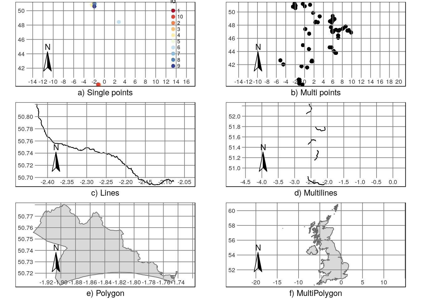
Vector layers consist of tables of data (attributes) together with descriptions of the geometries of the objects with these attributes. The geometries can be polygons, lines or points. There are also multi types for each of these. For example, the United Kingdom. See figure 1.1
## type is 19
Figure 1.1: Examples of vector data: Points can be either single (record of one occurence of a species) or multiple (all occurrences of a species). Lines can be held as either single features with corresponding to a name, e.g. the river Piddle, or multiple sections of a single river. Polygons can be either single (Bournemouth) or multiplygons (UK)
## [1] TRUE## type is 191.1.4.3 Map making and cartography
These are two traditional ways that GIS has been used. On screen digitising used to be the commonest use of GIS. Digitising involves drawing your own map, adding information, capturing and storing the results. This is the most obvious way to form an original map. Other methods involve geoprocessing or image classification. Digitising has become a slightly less important skill than it once was, due to the availability of online spatial data.
Cartography is the art and science of turning spatial information into useful products that display meaningful fool information. Maps are produced for a purpose. Many different maps can be developed from the same underlying information, each designed to show different aspects. Cartography is also a rather less important aspect of GIS than it once was, due to the growth of interactive web mapping. In section 2.3.2 you will see how easy it is to make modern webmap pages using R.
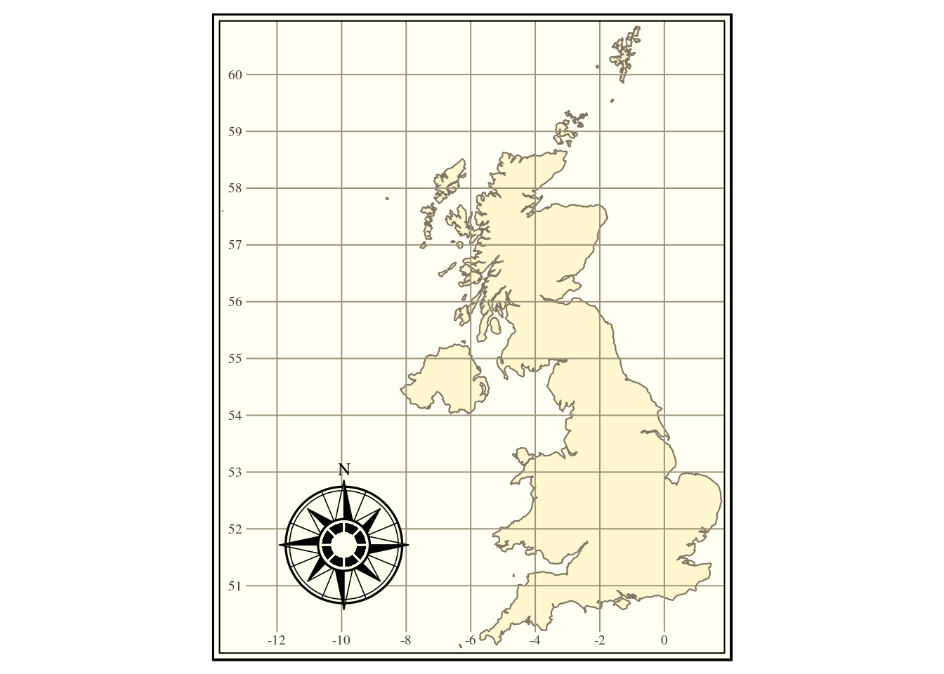
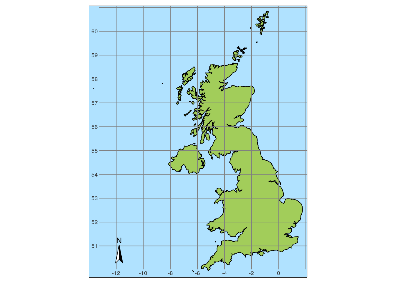
Some easy to use tools in R also produce maps which are designed with cartographic standards in mind. For example a very traditional “classic” style is applied in figure 1.2 and a simple “weather map” type style in 1.3. The tmap package also produces quick chloropleth maps. However cartography often tends to be rather a time consuming task, as it can be tricky to choose a way of displaying large amounts of information clearly in a non interactive map.

Figure 1.2: Map of the UK shown in a very traditional cartographic style

Figure 1.3: Map of the UK shown in a simple 1970s weather map type style
1.1.5 Exercise
Investigate some online spatial tools. For example
https://dopa-explorer.jrc.ec.europa.eu/dopa_explorer
Which elements of a GIS does this application use? What sort of data is being processed? How does spatial data (maps) link to temporal data (time series)? How important is good visualisation in allowing users to understand large quantities of data?