Section 2 Getting started: Projects and basemaps

2.1 Concepts

Most analyses in GIS combine data from multiple sources. Work is organised into project. A project file is simply a set of intructions that restores the software to the same state it was in when a project was saved. Organising work into projects saves a lot of time. Base maps are an essential element of any GIS project. Basemaps are obtained from streaming web services. You will be familiar with Google maps. If you have a Google account Google maps can be added to GIS projects as a base maps. However we will use only open source elements in this course. There are a large number of options that provide similar information to google maps.

2.2 QGIS: The GUI interface

The term GUI stands for graphical user interface. As GIS is a very visual form of data analysis using a GUI is a very natural way to work with geographical data. The interface to QGIS can be customised by the user to show different elements in different regions of the screen. You can add or subtract toolbars, change the panels which are visible using the menus at the top and move things around in many different ways. The screenshot below shows a basic default layout.

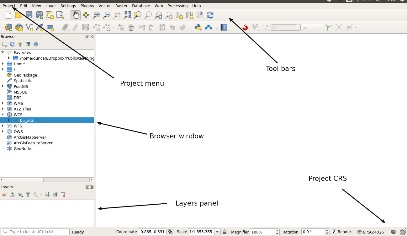
Figure 2.1: The elements of a QGIS graphical user interface: Note that the user can reconfigure all the visual elements so each interface may look different

You can install QGIS on your own laptop or PC from here.

https://qgis.org/en/site/forusers/download.html

2.2.1 Starting a QGIS project

The QGIS project file contains information regarding the CRS being used and the files that are loaded. Projects are used to restore QGIS to the state it was in when you were last using it. It is important to be aware that when you save a project you do not actually save the files themselves. A project typically uses one or more base maps as a backdrop to the information that will be processed.

Actions

Open QGIS

Notice that by default two of the most important panels that you will use are situated on the left hand side of the canvas. These are the browser and layers panels. If at any time these vanish you can restore them by looking for panels in the view menu. Most users customise their GUI in some ways. You can see a minor change that I make to the default interface in figure 2.2

To start a project in QGIS:

1. Click on the project tab in the top left hand side of the menu.
2. Find save in the menu
3. Save the QGZ file to a folder.

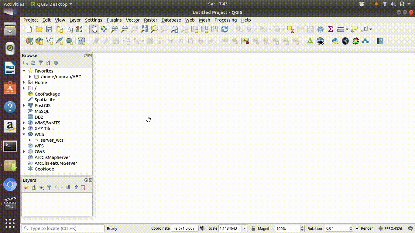
Figure 2.2: Starting a project in QGIS. Notice that browser and layers panels can be stacked to form a single tabbed panel. I think that this makes the interface easier to use, but each user has a different preference. You can customise your set up a little then save the project. Make sure that you know where the project is saved and that you keep the project and data files in the same folder. This example screenshot was taken on a Linux system

Take care when setting up a new project on the BU system. You must make sure that you know where your folder is situated. If you place all your data files plus the QGZ project file in the same folder, you can copy the whole folder onto a USB and open it in QGIS on your laptop. If the files are scattered across several folders this is not possible, and there is a danger that data will not be available to a project causing error messages and confusion.

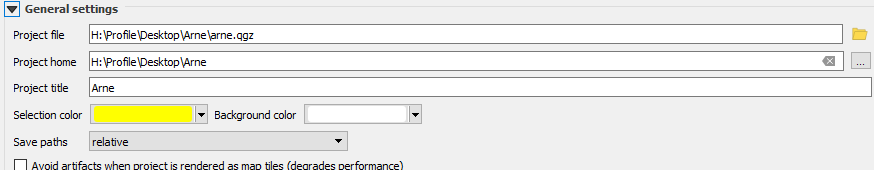
Figure 2.3: Do check your paths carefully on the BU system. Look in the project properties and set the projects home folder to the folder that contains your data. Don’t let the data and the project file become separated or you may not be able to restore the project easily. Notice that the save paths are relative by default, which means folders above the project file position will be recgnised, but those below may not. Take care

2.2.2 Adding base maps

In QGIS 3.2 adding base maps is achieved by selecting from the XYZ tile item in the browser tab. This should be preloaded with a set of useful options. However, if your PC does not yet have the basemaps preloaded, or if you are using your laptop you can load all the options by pasting this script into the python console (under the plugins menu).

https://raw.githubusercontent.com/klakar/QGIS_resources/master/collections/Geosupportsystem/python/qgis_basemaps.py

Actions

1. Click on the plugins menu tab.
2. Open the python console from the second menu option.
3. Move the focus to the web browser with the link above open
4. Press control A to select all the text.
5. Press control C to copy the whole script
6. Move back to the python console
7. Press control V to copy the text into the python console.
8. Press enter to run and wait for a few minutes for the installation to complete.

This all only needs to be run once.

Figure 2.4 shows all this in action.

Note that the animated gifs used in these documents run on a loop. They all last under one minute. You may need to watch for the start of the sequence.

Once the script has run through you will find a large number of base maps available under the xyz tab on the browser.

Figure 2.4: Adding xyz base maps to the QGIS interface: This operation only needs to be run once. Paste the script into the python console and press enter to run. Wait for a few minutes

You can make visualise the base maps by adding them to the canvas as shown in figure 2.5. Notice that the layers are added to the list of layers shown in the layers panel. The layer at the top of the list is visible at any one time. When a project is saved the list of layers which are open is also saved. You would usually only work with a single active base map at any one time, and it is simple to add new base maps whenever you want. A common combination is to open a cartographic layer such as Open Street map plus a satellite image.

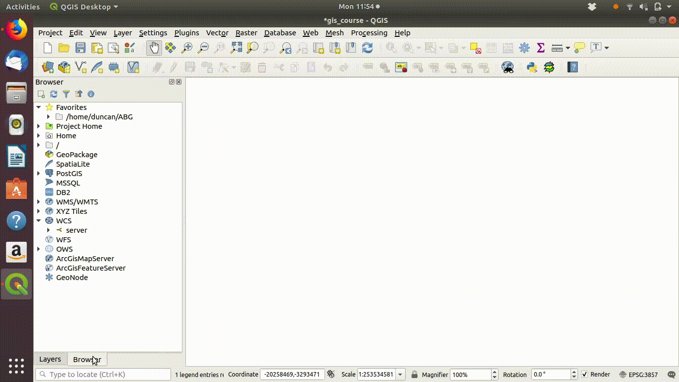
Figure 2.5: Adding xyz base maps to the QGIS canvas:

2.2.2.1 Exercise

Experiment with the base maps. Load several maps. Try reordering them in the layers panel and switching them on and off. Right clicking the name of the layer allows you to remove them.

2.3 Getting started in RStudio

Although the R language has been used for scripting GIS operations for well over a decade many users found it a difficult environment to work due to the lack of an interactive window for viewing the results of data analysis. This difficulty was largely resolved by the development of an R interface to the leaflet web mapping program. The mapview package further enhances this capacity by forming default web maps with one simple line of code.

2.3.1 Using RStudio

If you are completely new to RStudio this link may help you to get started.

http://r.bournemouth.ac.uk:82/books/AQM_book/_book/using-the-rstudio-server.html

Notice that RStudio also uses projects to organise work. A typical R GIS project would include a markdown script which makes interactive web maps and analyses data in a folder containing any data files that are used locally.

The BU RStudio server is currently running on http://r.bournemouth.ac.uk:8789/. The server is linked to the Postgis data base which provides access to many vector layers.

See section 4

2.3.2 Base maps in R

The most effective way to build up GIS analyses in R together with interactive maps displaying the results is to always use markdown documents as shown in the tutorial on the use of rstudio (http://r.bournemouth.ac.uk:82/books/AQM_book/_book/using-the-rstudio-server.html). Do take some time to work through this if you are still unfamiliar with markdown document concept. You will need to use markdown for web mapping and running interactive GIS in R. To use R for for GIS in the manner shown in this course you do not type commands directly into the R console. The workflow involves building up your analysis as a series of code chunks embedded in a markdown document and run in sequence. Then the document is knitted in order to produce maps and analytical results. This is the way all the course material that is contained in these worksheets has been produced. All the R code included will run on the BU server and produce the results shown.

The first code chunk in any markdown document should load the libraries needed for the analysis,

require(mapview)
require(rnaturalearth)

The next step is to obtain some data. For example, the rnaturalearth package has some simple maps at a global scale.

uk<- ne_countries(country = 'United Kingdom',scale=10)

Now a simple, default interactive map is produced by just enclosing the name of the object in the mapview command.

mapview(uk)

Notice that there are five base maps to choose from in the default configuration. You can flick through them by opening the square control in the top left corner of the web map. If you wish to add more base map options, or change the order of the base maps this can be achieved by changing the names in the mapview options.

mapviewOptions(basemaps =c("Esri.WorldImagery","OpenStreetMap","Esri.WorldStreetMap", "CartoDB.Positron", "OpenTopoMap", "OpenStreetMap.BlackAndWhite", "OpenStreetMap.HOT","Stamen.TonerLite", "CartoDB.DarkMatter", "Esri.WorldShadedRelief", "Stamen.Terrain"))

mapview(uk,alpha.regions = 0)

2.3.2.1 Exercise

Start a new project in the RStudio server. Open a markdown document and save it under a new name.

Add the code chunks shown above to form a web map and knit the document.

Experiment with some different base maps by carefully altering the mapview options.

Care with syntax If you are new to using R do be aware that seemingly minor changes to the syntax of a chunk of code can prevent the code from working. This is common to all computer languages and can be frustrating at the start. All the code for this course will run as is, providing the code chunks are run in the correct order and the packages are all loaded.

2.3.3 Screenshots of a new user starting their first web map in R

These screenshots show a new user trying RStudio. Notice the steps needed to make a web map.

1. Start a new project in a new directory.
2. Open a new markdown document
3. Change the content of the markdown document by pasting in code chunks.
4. Annotate the document.
5. Run chunks sequentially to test them
6. Knit and save the document.

This produces an HTML web map that can be saved and used off the server even if layers from the server are included.

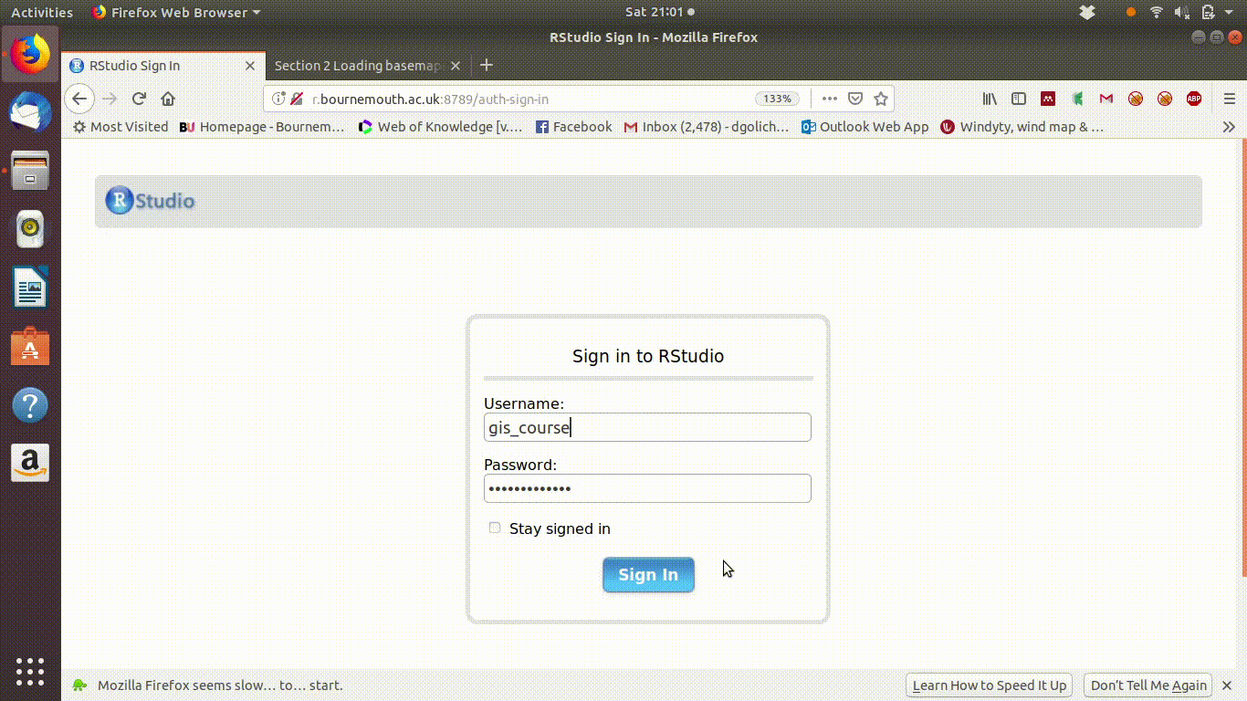
Figure 2.6: Logging on to the RServer as user GIS_course and starting a project in a new directory. You should use a new project and a new directory for each analysis. A project may include several files within the same directory. These course notes are all compiled within a single project.

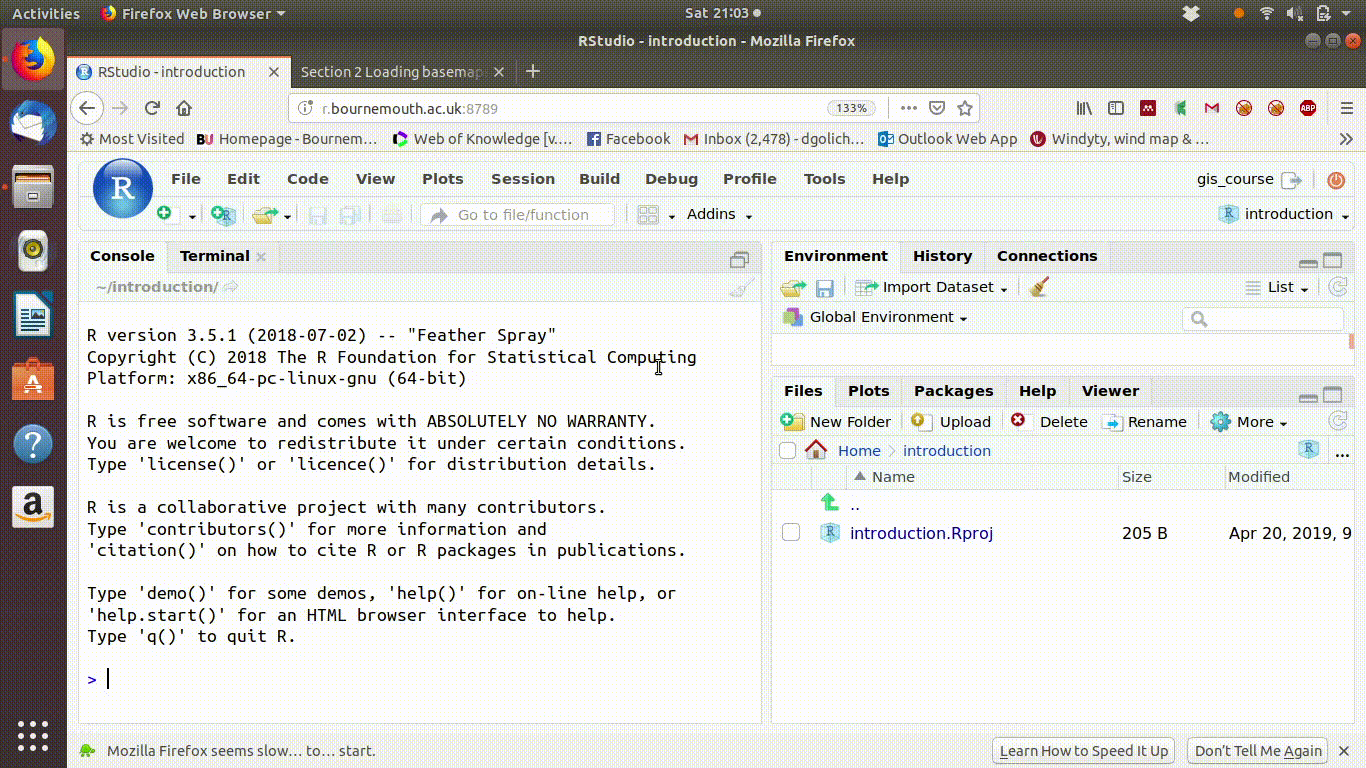
Figure 2.7: Starting a new markdown file. The default file is a demo which contains code to make a histogram and do some simple stats. This code needs to be deleted as we are starting from scratch. The default titel is untitled and the default file name is untitled. Save the file with a new name and type in a title for the finished document.

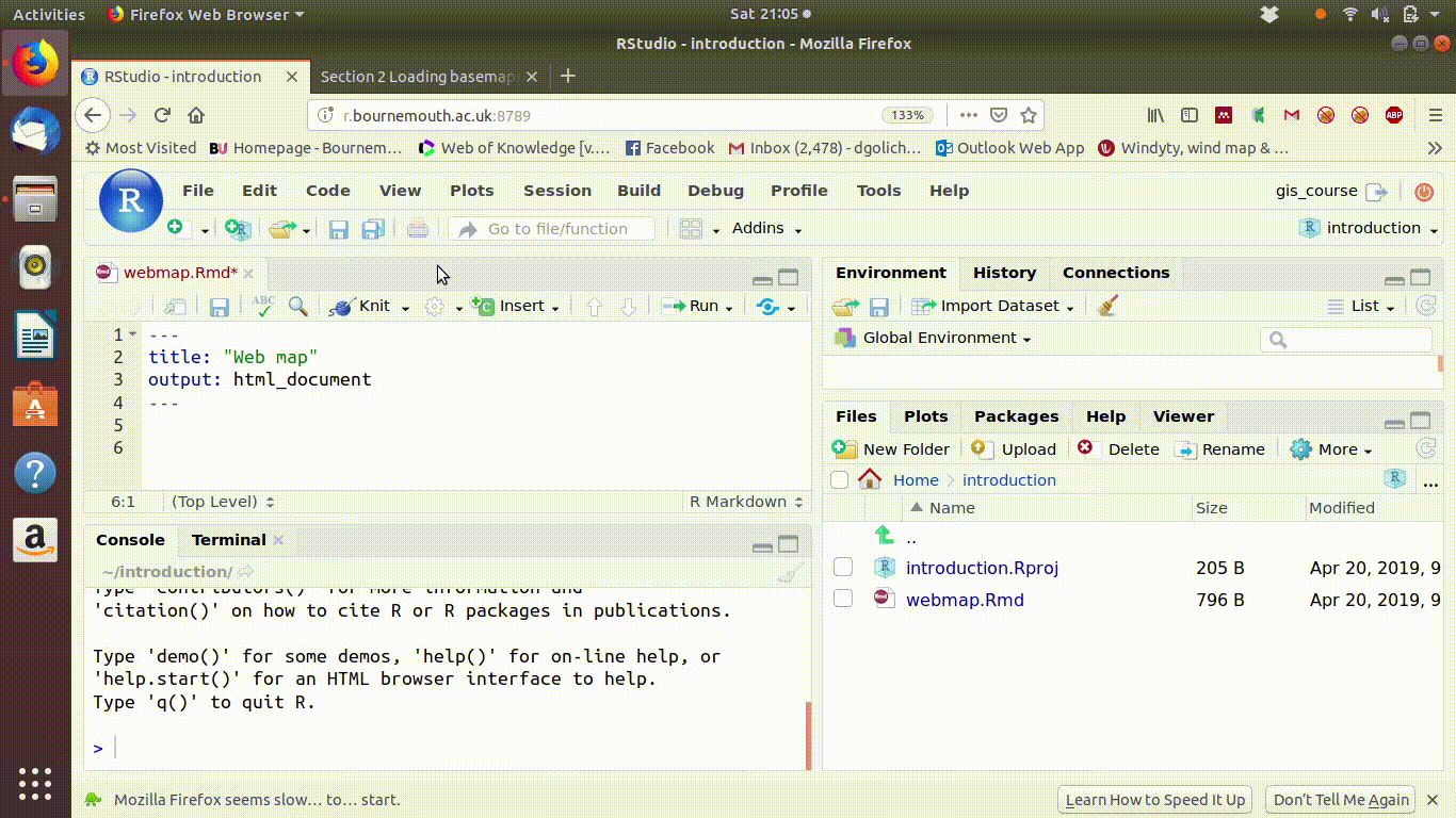
Figure 2.8: Pasting code in from the course web site. Keep both tabs open and make sure that the code is followed exactly as it is shown in the book. Insert a code chunk, copy the code shown, paste it in then press the run button. This may seem odd at first, as nothing seems to happen. However it is part of building up the script

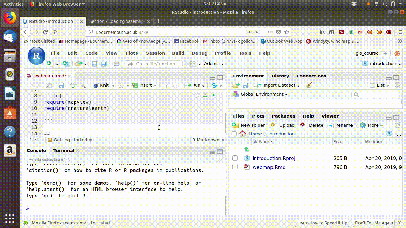
Figure 2.9: Adding another section. Clearly the first time you try this it will all seem mysterious. Nothing seems to be happening and there is no obvious interface. This is a different way of working that needs time to adjust to. You are building a simple script that will turn into a web page. Make sure that you copy the code in the right order and that the script looks like the orginal in these course handouts.

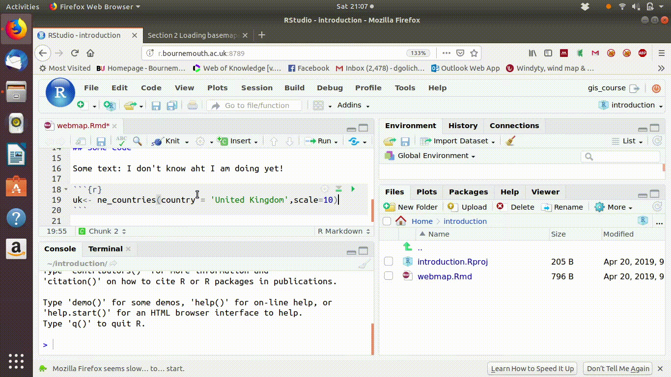
Figure 2.10: Paste each piece of code into a new chunk carefully. Press the arrow buttons on the code chunks to run both all the chunks above and to run the code chunk. This will make sense as soon as you have run a few analyses, but at the start it seems odd. Always type comments between each code chunk, even if they are only notes to yourself.

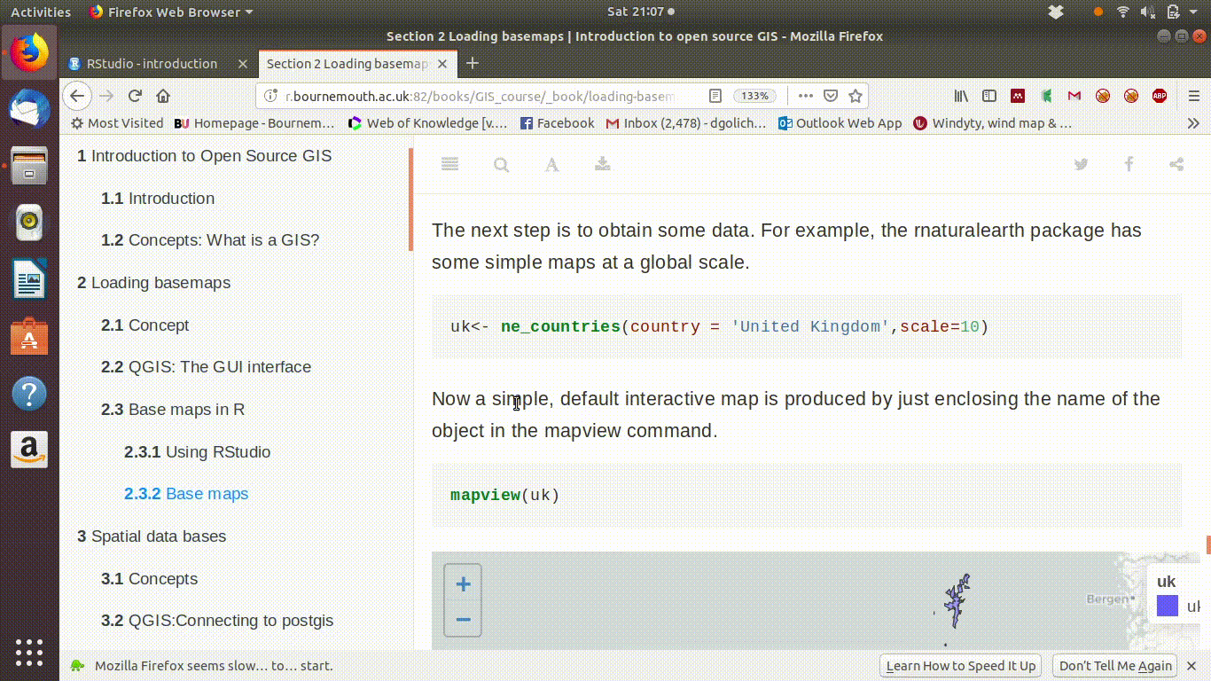
Figure 2.11: The first two code chunks set up the session. Now when a piece of code is pasted in that forms a map using the package that was loaded in chunk one and the data that was loaded in chunk two something does happen. A map appears in the output.

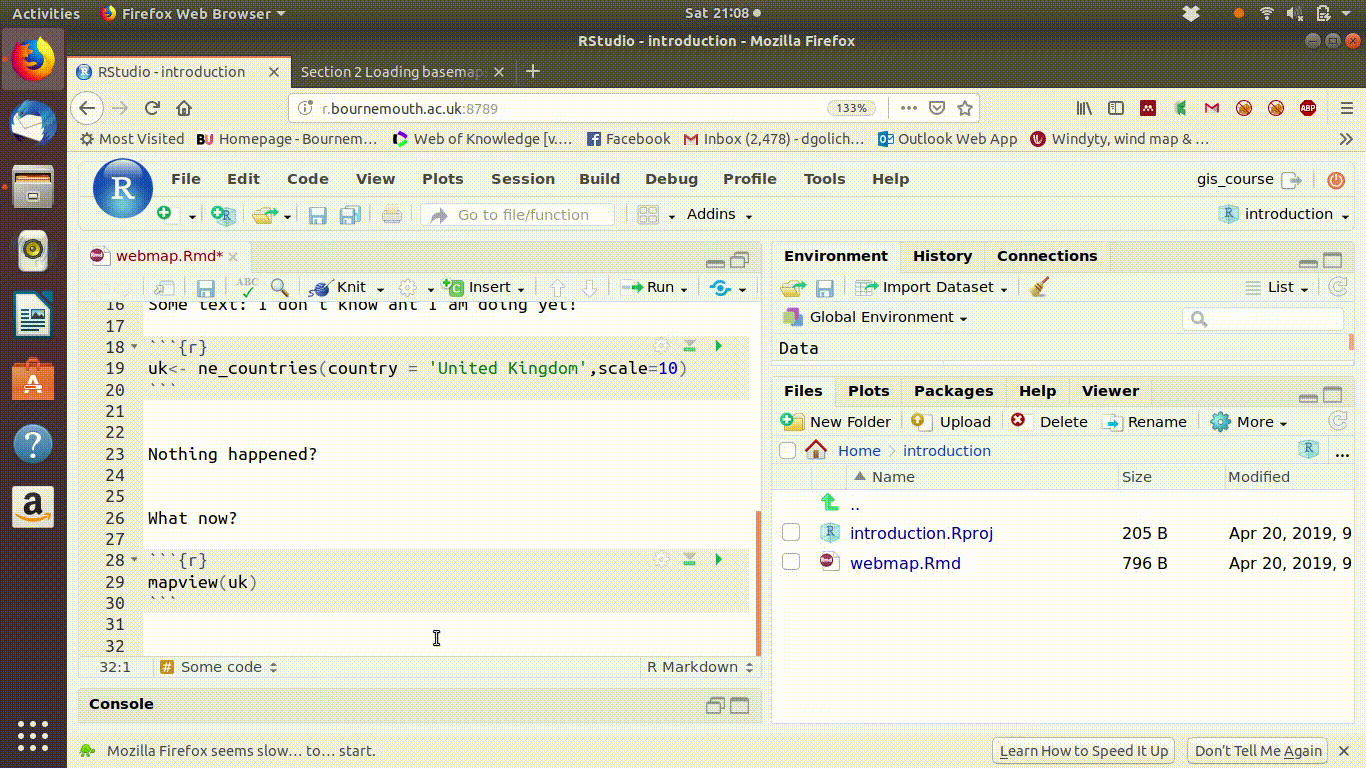
Figure 2.12: A map appeared and can be closed by clicking on the cross in the corner. Now what do we do?

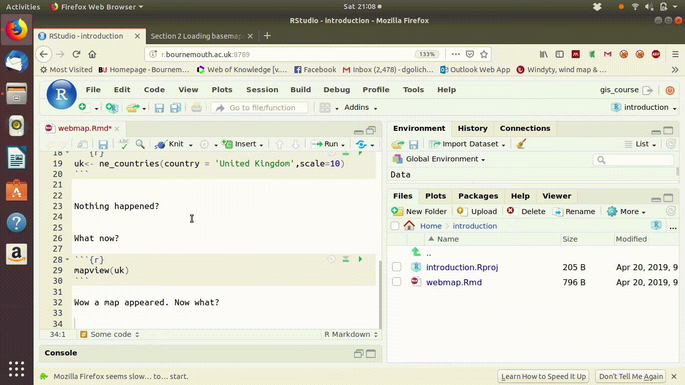
Figure 2.13: The answer to the last question is to knit the document to HTML. This forms a document with code and output embedded. The HTML file can be saved locally and used off the server as a web map. If analysis is carried out it will all be shown and can be added to a map that can be shared with others as a portable web page.