Section 14 Large raster layers
14.1 Concepts
Processing and analysing very large raster layers (i.e. fine grained layers with a broad extent) can be challenging. Methods that are very straight forward to apply to small rasters don’t always scale up. The problem with raster layers is that the dimensions are squared. This leads to a rapid increase in file size as regions become larger. Moores law states that processor speeds, or overall processing power for computers, tends to double every two years. This has been largely true over the last decade, so processing large rasters has become simpler over time. One of the side effects of Moore’s law has been that researchers often want to use results from projects that have used cutting edge processing power to form very large data sets. Large raster layers require special techniques for processing and visualisation. In a research context algorithm can be implemented on large raster layers that take days to run. In this introductory course we will focus on the use of subsets taken from large rasters at a local level.
There are two challenges involved when working with large raster layers. The first issue involves visualising the data This is relatively easily resolved through techniques such as “pyramiding”. This adjusts the resolution at different zoom levels. Software such as Geoserver automates this. The ease with which visualisation is achieved can hide the second issue, which is the important one in the context of data analysis. Just because you can see large raster layers in a GIS or web map in real time, it does not imply that you can run an analyses on them quickly.
The second challenge is the result of the actual quantity of information that has to be processed if an analysis is conducted on a whole large raster layer. For example, the Lidar based terrain analysis that we implemented in just a few seconds at the site level in section 10 would take many hours to run through at 2m resolution for the whole county of Dorset. If an operation has to use a PCs working memory it may easily hang or crash. This can be very frustrating.
14.1.1 Visualising a large raster layer
A good example of a very large raster visualisation on the web is found here.
https://earthenginepartners.appspot.com/science-2013-global-forest
This on-line “slippy” map can be zoomed and panned very quickly to look at patterns of deforestation. It is using WMS (or similar) to ensure that the pixel resolution changes to match the zoom level.
However to run a bespoke analysis of this data set we will need the raw data. The data tiles can be downloaded as granules from this link
https://earthenginepartners.appspot.com/science-2013-global-forest/download_v1.6.html
The gain, lossyear, and datamask layers total less than 10GB each globally. However the treecover2000 layer totals around 50GB. This is a large data set, which was derived originally from a much larger one consisting of terrabytes of Landsat imagery.
14.1.2 Using a geoserver to cut out site level data
The exercise below could be the start of a research project at a tropical forest site. If we are interested in a protected are of tropical forest we would certainly want to obtain Hansen’s analysis for the area of interest in order to check the veracity of the classification and incorporate the data layer in an analysis. One way to do this would be to go through the process of downloading the granules individually. A more efficient approach is to do this on a server. That makes the data easily available to all users without rerunning tedious downloads and clipping.
All Hansen’s data layers have been downloaded and placed on the BU geoserver. The files have been mosaicked to form a single seamless coverage.
The geoserver is part of a stack of software that is used in web mapping. The architecture is shown in figure 14.1
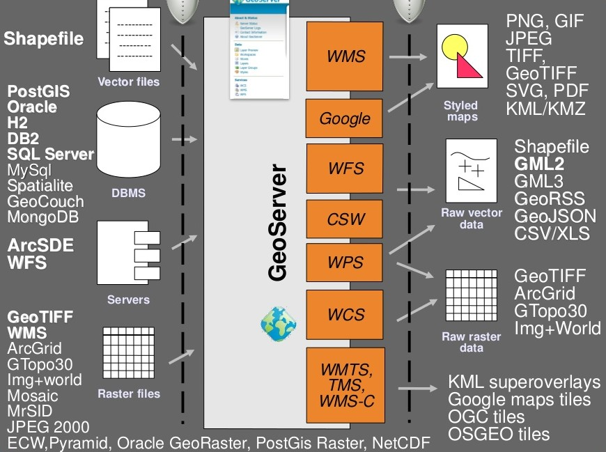
Figure 14.1: Architecture of a system using a Geoserver
Notice from figure 14.1 that postgis is linked to the Geoserver. This link can be used to pass data held in a data base to web maps safely and securely, without giving out log in details. The main purpose of this is to use WMS to visualise the data.
14.2 Connecting to the geoserver using QGIS
The BU WCS and WFS geoserver connections are only available on campus, for obvious reasons. They run through the URL 172.16.49.31. The port used for the geoserver is 8083. There is an off campus WMS connection (see section 14.3.2)
14.2.1 WMS connection
The Web Map Service (WMS) serves pictures of the raw data, rather than the data themselves in the original format. This is not useful for local processing. However it does provide fast visualisation of the layers and can be queried to find some information.
Setting up the connection is a simple process.
Action
- Right click the WMS/WMTS tab in the browser panel.
- A window will open for connection details.
- Give the connection any name that you can remember (I’ve used server_wms here)
- Copy and paste (or type carefully) the following URL http://172.16.49.31:8083/gis_course/wms?
- Save and close and the connection is established. Figure 14.2 shows this in action.
Figure 14.2: Setting up a WMS connection in QGIS.
14.2.1.1 Loading WMS layers
Once the connection is set up the layers can be loaded by dragging and dropping onto the canvas. There is no need to worry about the size of the data with WMS. It is designed for visualisation.
Figure 14.3: Loading layers from the WMS connection: This simply involves dragging and dropping the layers onto the canvas
14.2.1.2 Setting up a WCS connection
You must take much more care when using WCS than with WMS. WCS is potentially rather dangerous, as it allows all the raw data to be transferred over a network. If you have tried downloading one of the tiles from Hansen’s site you will appreciate that you certainly would not want QGIS to attempt to download all of them at once.
Setting up the connection is a similar process. This time use URL http://172.16.49.31:8083/gis_course/wcs? See figure 14.4
Figure 14.4: Setting up the WCS connection.
14.2.1.3 Loading WCS layers
Once again, loading the layers is very easy, but this is the point at which things can potentially go badly wrong if you don’t take care. Loading a WCS sends the command to the geoserver telling it to transfer all the raw data for the area being viewed. If too much data is requested at a time the system could hang.
14.2.1.4 Saving WCS layers
You also need to take care when saving WCS layers.
Action
- Load the WCS forest2000 and loss layers when zoomed to a sensible extent. The example below uses the polygon for the Giam Siak Kecil reserve. This can be added by making a connection to a data base in postgis and running a query (see 14.3.0.1)
- Load the forest2000 and loss layers to the canvas.
- Right click each layer, choose export and save locally.
- Make sure that you select the map canvas extent when saving. This is very important!
Figure 14.5: Loading the WCS layers. Always zoom in to the local area of interest before trying to load WCS. Notice that in this example the layers load quickly and you can start the process of saving them locally within a few seconds. Larger layer can take many minutes.
14.2.1.5 Cleaning up
Always remove the WCS connection before going any further. Accidentally zooming out with the WCS still connected will mean that data is loaded again.
Figure 14.6: Tidy up by removing the WCS layers after saviing locally. The WCS
14.3 R: Processing large raster layers
If we were designing a tool such as a Digital Observatory for Protected Areas we would want any analysis that we conducted on a single reserve to be potentially reproducible across all the reserves held in the world data base of protected areas. This is a “big data” project that has been carried out recently. The results are made available through this excellent web portal.
https://dopa-explorer.jrc.ec.europa.eu/dopa_explorer
In this section will look at how R can reproduce this type of analysis.
require(giscourse)
require(RPostgreSQL)
require(rpostgis)
require(sf)
require(mapview)
require(leaflet.extras)
require(raster)
mapviewOptions(basemaps =c("Esri.WorldImagery",
   "Esri.WorldShadedRelief", "Stamen.Terrain"))
14.3.0.1 Loading a single reserve polygon from wdpa
Let’s find the forest cover change around a reserve in Indonesia.
We will begin by loading a single polygon representing a protected area from the world data base of protected areas.
https://www.protectedplanet.net/
This has been added to a BU postgis data base (note that the layer is not placed in the gis_course data base as the intention was to keep the size of the course data base limited).
conn <- connect("clima2")
reserve<-st_read(conn, query = "select gid,name,geom from wdpa where name ='Giam Siak Kecil'")
plot(reserve$geom,axes=TRUE)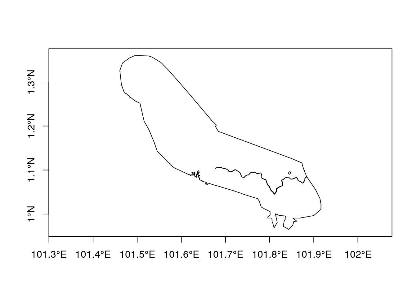
dbDisconnect(conn)
#> [1] TRUE
14.3.1 Terrain analysis
We can reuse the code from previous chapters to quickly visualise the terrain around this reserve.
library(elevatr)
elev <- get_elev_raster(reserve, z = 9,clip="bbox")
elev <- projectRaster(elev, crs=st_crs(reserve)$proj4string) ## Make sure we stillknow the CRS
elev[elev<0]<-NA
elev[elev>100]<-NA

slope<-terrain(elev, opt='slope', unit='degrees')
aspect<-terrain(elev, opt='aspect',unit='degrees')
sloper<-terrain(elev, opt='slope', unit='radians')
aspectr<-terrain(elev, opt='aspect',unit='radians')
hillshade<-hillShade(sloper,aspectr,angle=5)hist(elev)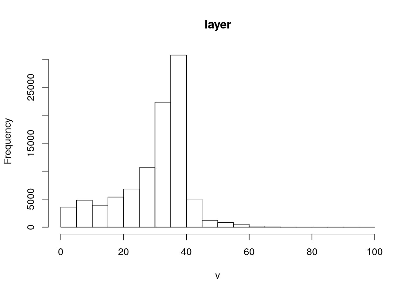
plot(hillshade, col = gray(0:100 / 100), legend = FALSE)
plot(elev, col = terrain.colors(25), alpha = 0.4, legend = TRUE, add = TRUE)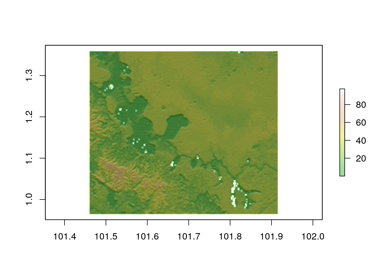
14.3.2 Adding WMS tiles from the BU geoserver
The leaflet extras package is needed to add WMS layers to mapview maps. This involves quite a few lines of code, so they have been wrapped up into a wrapper function in the course code package.
hansen_wms<-function(m){

  require(leaflet.extras)
  require(mapview)
  m@map %>% addFullscreenControl() %>% addMiniMap(position = "bottomleft",zoomLevelOffset = -4, toggleDisplay = TRUE) %>%
    addWMSTiles(group="Forest 2000",
                "http://r.bournemouth.ac.uk:8083/gis_course/wms",
                layers = "gis_course:forest2000",
                options = WMSTileOptions(format = "image/png", transparent = TRUE)) %>%
    addWMSTiles(group="Forest loss",
                "http://r.bournemouth.ac.uk:8083/gis_course/wms",
                layers = "gis_course:loss",
                options = WMSTileOptions(format = "image/png", transparent = TRUE)) %>%
    addWMSTiles(group="Cover gain",
                "http://r.bournemouth.ac.uk:8083/gis_course/wms",
                layers = "gis_course:gain",
                options = WMSTileOptions(format = "image/png", transparent = TRUE)) %>%
    mapview:::mapViewLayersControl (names = c("Forest 2000","Forest loss","Cover gain")) -> mymap
return(mymap)}mapview(reserve) %>% hansen_wms()This is great for looking at the data, but its a WMS so we can’t do anything with it directly.
14.3.3 Accessing the raw data
When working on raster data directly that is held on a server there is no need to pass it through a geoserver. Data can be manipulated more quickly directly within the file system.
Hansen’s layers are in three directories on the server.
A script was used to automatically pull down all the layers from the without clicking on each one in turn. The script takes advantage of the consistent file naming conventions on the site to loop through all the options that are needed.
See ?? for example of downloading using wget.
14.3.4 Building a VRT to reference all the data files
A very useful trick when working on large rasters held within a local (to the server) file system is to build a virtual raster catalogue (vrt). This takes just a few seconds using gdal, even for hundreds of files. The VRT simply references the file names and checks that all the data is in the same format and at the same resolution.
path<- "~/geoserver/data_dir/rasters/hansen2018/forest2000"
system(sprintf("gdalbuildvrt ~/geoserver/data_dir/rasters/forest2000.vrt %s/*.tif",path))
path<- "~/geoserver/data_dir/rasters/hansen2018/loss"
system(sprintf("gdalbuildvrt ~/geoserver/data_dir/rasters/loss.vrt %s/*.tif",path))
path<- "~/geoserver/data_dir/rasters/hansen2018/gain"
system(sprintf("gdalbuildvrt ~/geoserver/data_dir/rasters/gain.vrt %s/*.tif",path))
14.3.5 Referencing the data as raster layers in R
The next part of the process is also extremely quick to run, as nothing is actually loaded. It involves setting up the vrt layers as rasters in R.
library(raster)
ghs<- raster("~/geoserver/data_dir/rasters/ghs/gdal_ghs2.tif")
forest2000 <- raster("~/geoserver/data_dir/rasters/forest2000.vrt")
loss <- raster("~/geoserver/data_dir/rasters/loss.vrt")
gain <- raster("~/geoserver/data_dir/rasters/gain.vrt")
Do not try to process these vrts without cropping to a local area! The VRT contains a reference to all the data on the server. This would hang the system.
14.3.6 Cropping to the reserve
Once these references are set up, sub-setting the large data set is reasonably simple. The CRS is 4326 however, so transformations are required in order to work with distances in meters. We’ll transform into web mercator and then take an area within 10km of the reserve boundary.
res3857<-st_transform(reserve,3857) #Transform
buf10km<-st_buffer(res3857,10000) # Buffer to 10 km
sarea<-st_transform(buf10km,4326) # Retransform for the clipping
forest2000<-raster::crop(forest2000,sarea)
loss<-raster::crop(loss,sarea)
gain<-raster::crop(gain,sarea)
14.3.7 Reprojecting raster layers
It is simpler to work with reprojected raster layers.
## Reproject all the rasters
forest2000 <- projectRaster(forest2000, crs=st_crs(res3857)$proj4string)
loss <- projectRaster(loss, crs=st_crs(res3857)$proj4string)
gain <- projectRaster(gain, crs=st_crs(res3857)$proj4string)
We can check the resolution (pixel dimensions)
res(forest2000)
#> [1] 27.8 27.8
So we have the area in square meters of each pixel.
pix_area<-prod(res(forest2000))
pix_area
#> [1] 772.84
14.3.8 Calculating the area lost
It is now possible to calculate the precise area lost (according to Hansen’s classification) each year for the area within the reserve and the area in the 10km buffer around the reserve. To do this we just need to mask the raster using each polygon then tabulate the number of pixels in each class. A couple of extra lines in R calculate the area in hectares and the percentage of the total area.
loss_in<-raster::mask(loss,res3857) #Mask
area_in<-as.numeric(st_area(res3857)/10000) #Get total area of reserve

d<-data.frame(table(round(getValues(loss_in),0))) # Tabulate the results


d %>%
  mutate(area_ha=Freq*pix_area/10000) %>%
  mutate(percent=round(100*area_ha/area_in,1)) %>%
  mutate(year=as.numeric(as.character(Var1))+2000) %>%
  mutate(region="Within")->d
Pixels that were not lost have values of zero. The non zero values represent the year of loss begining in 2001.
Repeat this for the area around the reserve.
around<-st_difference(buf10km,res3857)
area_around<-as.numeric(st_area(around)/10000)

loss_around<-raster::mask(loss,around)
d2<-data.frame(table(round(getValues(loss_around),0)))

d2 %>%
  mutate(area_ha=Freq*pix_area/10000) %>%
  mutate(percent=round(100*area_ha/area_around,1)) %>%
  mutate(year=as.numeric(as.character(Var1))+2000) %>%
  mutate(region="Around")->d2


d<-rbind(d,d2)library(dplyr)
library(ggplot2)
d %>% filter(year>2000) %>% ggplot(aes(x=year,y=percent,col=region)) +geom_line() +ylab("Percent of total area deforested per year")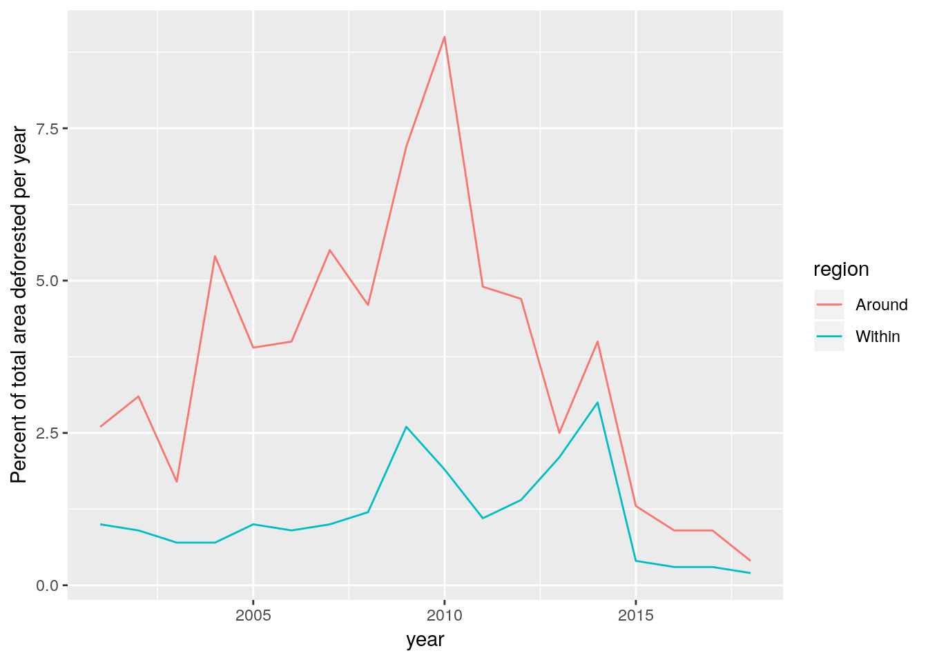
d %>% filter(year>2000) %>% ggplot(aes(x=year,y=cumsum(percent),col=region)) +geom_line() +ylab("Cumulative deforestation as percentage of total area")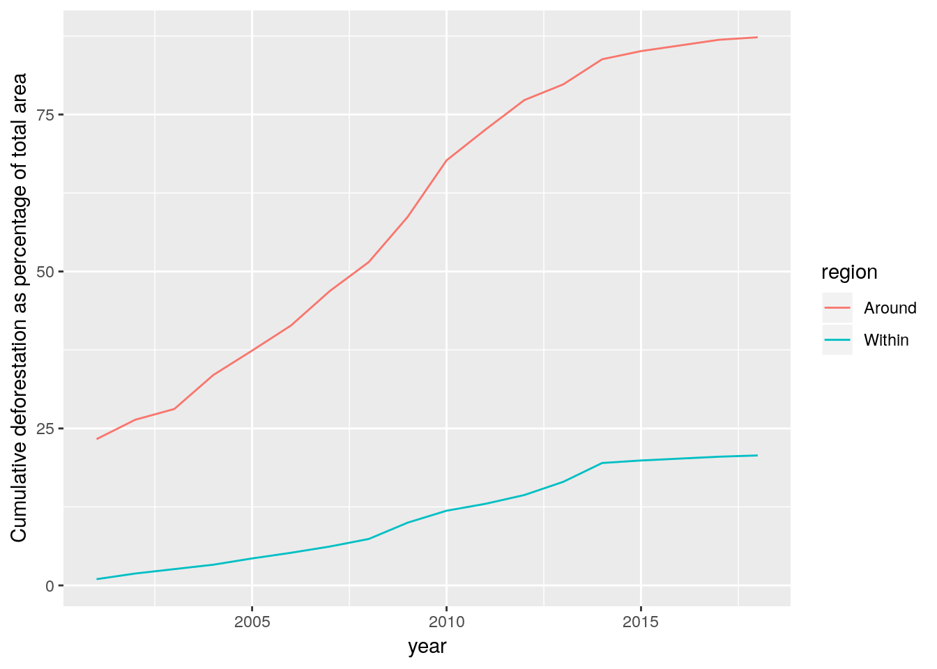
14.3.9 Exercises
Techniques such as map algebra can now be applied to the data layers. They can also be visualised as web maps and turned into other cartographic products. Design a piece of research based on these data, or select data from another area following the same protocol.
dbDisconnect(conn)
rm(list=ls())
lapply(paste('package:',names(sessionInfo()$otherPkgs),sep=""),detach,character.only=TRUE,unload=TRUE)