Section 9 Geoprocessing

9.1 Concepts

Geoprocessing is the term given to any operation that alters the geometry of spatial data. An example of geoprocessing has already been shown, in section 7.3.4. There are many books and web bages that show details of the common vector geoprocesing operations, often in the form of venn diagrams. These won’t be repeated here. A good, comprehensive description of geoprocessing with R code to run it is provided by Lovelace’s book.

https://geocompr.robinlovelace.net/geometric-operations.html#geo-vec

The wide range of possible geoprocessing operations might give the impression that geoprocessing provides lots of different answers in search of a problem. Geoprocessing is used very frequently when doing GIS. Sometimes it is a principal analytical method but it is also often needed in order to sort out rather mundane issues such as minor topological errors and generally put the geometry into shape ready for further analysis.

Geoprocessing can be applied whenever a change to the geometry of the layers you are interested in can be achieved by applying a rule or a set of rules.

The alternative to geoprocessing is to edit the layers manually. This may be necessary if you can’t find a rule that does the job that you want. However it is usually much more time consuming.

The geoprocessing toolbox is the general problem solving workshop of vector GIS. It is quite difficult to teach the use of geoprocessing. Every problem that arises tends to be different in nature. Geoprocessing tools usually have to be used in a series of steps. As you learn what geoprocessing does it becomes increasingly easy to implement these steps and choose a method that will fix a problem you have. Using R scripts or postgis makes the steps quick and reproducible. Postgis can be used directly for server side geoprocessing on very large data sets.

Think carefully when running geoprocessing operations. It is important to be aware of the connection between the attribute table in the original layer(s) and the new geometry. As geoprocessing works on the geometry the match between geometry and attributes often breaks down. In particular, areas and lengths usually have to be recalculated.

9.2 QGIS

Although geoprocessing is best achieved using code, the QGIS GUI produces visual output quickly and easily. It is very useful when learning geoprocessing techniques as the results can be seen quickly.

Geoprocessing in QGIS became much easier when the program introduced temporary scratch pad layers. This is a great feature of QGIS. A series of operations can be built up using intermediate temporary layers without the need to save each one. This avoids filling a project folder with unecssary layers. However always remember that the layers are temporary and will be lost if not saved.

The geoprocessing tools are found as the first element below the vector heading on the top menu of QGIS (they can also be found in the toolbox if that is open).

If you are new to the concept it is well worth opening the menu and browsing the tools. Each one has a clear textual description of what it does along side. There is no point in repeating this text here.

Let’s put geoprocessing to use.

Action

1. Load the Arne priority habitat layer from the Arne schema produced by the code in section 7.3.4 from the postgis connection.
2. Right click on the layer to open the properties menu
3. Go to symbology and choose categorized (not shown in the figures below)
4. Shade the layer using the main habitat category.

Figure 9.1: Shading the Arne priority habitats layer. Choose random colours based on the category. If the layer is going to be used for cartography the choice of colours would be important, but it is not so critical when you are just working on an analysis.

Figure 9.2: Add some basemaps and check the alignment of the priority habitats with features on the ground.

Figure 9.3: Zooming in to compare the priority habitat delimitation.

Action

1. Inspect the layer with relation to some base maps. Zoom in and out. Notice that the priority habitats are divided into sites. For many uses this is NOT what we want.

A problem to solve

For many purposes it would be preferable to join the elements together to form a continuous layer with no breaks. This is an issue that geoprocessing can solve. The idea is to dissolve the geometry in order to simplify it.

1. Click on the geoprocessing tools and find the dissolve option
2. Dissolve the geometry using the main habitat field as the input.
3. Click run
4. Right click the parent layer and find copy style. Copy the style to the clipboard then paste it into the new map style.
5. Look at the results

These steps are all shown in figure 9.4

Temporary scratch layers are used for each step of the analysis which are lost when the program is closed. This is very much a feature, not a bug. It is far simpler to discard all intermediate steps in an analysis than to fill a folder with saved layers.
However always remember to save the final layer!

Figure 9.4: Dissolving the priority habitats layer on the main habitat attribute. Go to the vevtor menu, choose dissolve then make sure that the main habitat attribute is selected. Click run. The figure also shows the style being copied to the new layer.

Notice that the style from the parent layer is being copied to each of the new layers. You can do this by right clicking the layer, copying the style and then choosing paste style. This is a convenient way to make sure that the colour schemes of each of the layers match up so you can check the results..

In figure 9.4 you can see the results of the dissolve operation. Most of the dividing lines between the habitats have been dissolved. The divisions based on paths are still present. However there are still a few odd slivers and unwanted lines.

Figure 9.5: Pasting the style into the dissolved layer and looking at the results by switching between the original and the dissolved layer

Although dissolving the layers has produced more or less the result we expected, there are still a few unwanted lines. A trick to clean up these is to run a very narrow buffer. This is shown in figure 9.6 and figure 9.7

Figure 9.6: Using a very small buffer to clean up a dissolved layer: This trick is often useful

Figure 9.7: .

9.2.1 Buffering and differencing

A common operation is to find all the features beyond a certain distance from others. For example all the habitat at Arne that is further than 50 meters from paths. This is a simple buffer operation followed by differencing.

Action

1. Load the paths layer from the Arne schema.
2. Run a 50m buffer around it. See figure 9.8
3. Take the difference between the habitat layer and the buffered paths See figure 9.9
4. Inspect the results figure 9.10

Notice that when running a buffer you often choose to dissolve the results. This is can be a good idea as it produces a simpler layer. In this case it doesn’t alter the final result that is provided by the differencing operation. You may want to experiment with this.

Figure 9.8: Forming a 50m buffer around the paths

Figure 9.9: Taking the difference between the paths buffer and the

Figure 9.10: Looking at the results of the buffering and differencing

9.3 R: Geoprocessing using postgis and R

knitr::opts_chunk$set(echo = TRUE,eval=TRUE)

library(giscourse)
conn <- connect()

Once you have learned enough about geoprocessing operations to know how they can be used, actually implementing geoprocessing can be much quicker using postgis than QGIS.

The data structure and the functions in the sf (simple features) package in R match those in postgis in many respects.

query1<-"select mhabitat,st_buffer(st_union(geom),0.1) geom 
from arne.phabitat group by mhabitat "
habitat<-st_read(conn,query=query1)

The burst option in mapviews can be useful when looking at a layer with a smallish number of categories, as this allows each one of the categories to be made visible or invisible separately.

mapview(habitat,zcol="mhabitat",burst=TRUE, legend=FALSE,zoom=FALSE)

The paths buffer query can also be run in postgis.

query2<-"select st_buffer(st_union(geom),50) geom 
from arne.paths"
paths<-st_read(conn,query=query2)
qtm(paths)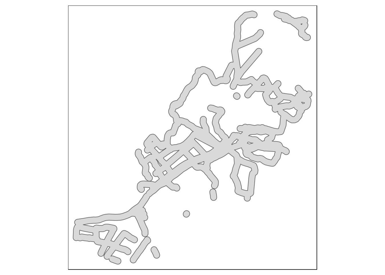

9.3.1 Joining subqueries using sprintf

The sprintf trick is particularly useful when building a chain of geoprocessing steps into a single query.

query3<-sprintf("select mhabitat,st_difference(h.geom,p.geom) 
    geom from (%s) h, (%s) p",query1,query2)

This trick saves having to type out all the text of each subquery again, which could easily result in a syntax error. Notice the way sprintf uses %s to represent strings that are replaced by the text in query1 and query2. This is the resulting query. It looks quite complex when all the text is placed together, but effectively this conducts all the operations that were demonstrated in QGIS in one shot in postgis.

select mhabitat,st_difference(h.geom,p.geom) geom from (select mhabitat,st_buffer(st_union(geom),0.1) geom from arne.phabitat group by mhabitat ) h, (select st_buffer(st_union(geom),50) geom from arne.paths) p

One way to learn how to construct queries like this is to experiment with small layers such as those in the Arne schema in the db manager of QGIS.

dif<-st_read(conn,query=query3)
qtm(dif,"mhabitat") +tm_style("classic")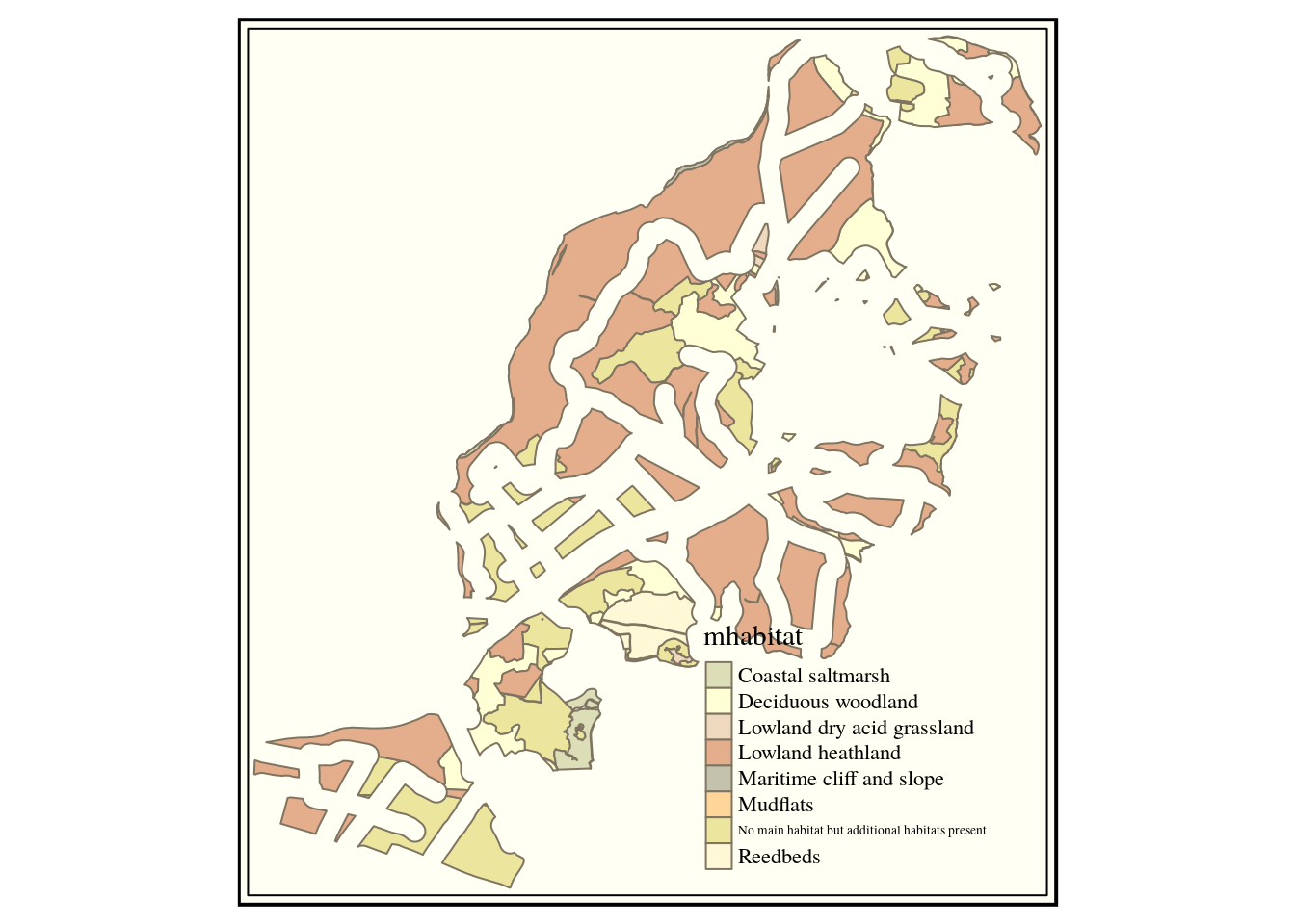

Do not attempt to run geoprocessing queries or any other complex operations in postgis on large data tables such as the original priority habitat layers until you are more experienced. A key advantage of postgis is that it is possible to run analysis on very large data sets. In theory all the priority habitat patches further than fifty meters from all the paths in Dorset could be extracted from the data with one query. In practice this query could take hours to run through, so techniques involving prototyping are needed for big data operations. See section x on big data operations in postgis (which I have not written yet!)

9.4 Calculating areas after geoprocessing

To summarise the series of operations.

1. The priority habitat layer was dissolved to unite all the areas with the same main habitat classification.
2. A buffer of 50m was produced around the paths in the study area.
3. This buffer was subtracted from the unified priority habitat map.

So the difference layer holds all the habitat patches that are further than 50m from a path. We can now easily find out the total area of these classes of habitat both before and after the differencing.

library(dplyr)
habitat$total_area_ha<-round(st_area(habitat)/10000,1)
dif$core_area_ha<-round(st_area(dif)/10000,1)

habitat %>% st_set_geometry(NULL) -> d1
dif %>% st_set_geometry(NULL) -> d2

left_join(d1,d2, by = "mhabitat") %>% DT::datatable()

9.4.1 Multi polygons to single polygons

The table pf results had one row for each habitat type. This was because the SQL geoprocessing query had grouped the results by main habitat class leading to a multi geometry column. If we wanted to know the area of each polygon we need to cast the multipolygon to single polygons.

dif %>% st_cast("POLYGON") -> dif2
dif2$area_ha<-round(st_area(dif2)/10000,1)

mapview(dif2, zcol = "mhabitat", burst=TRUE,legend=FALSE)

9.4.2 Reproducing the same analysis for a different site

The big advantage of using R lies in the reproducibility of all the analyses. Although it may have taken some time to develop an analysis for Arne it can now easily be used in a different setting.

What if we want to move the focus to Hengistbury head? This is a local nature reserve with a polygon delimiting the boundary in the local_reserves table. So the query below which just drops in the new area will do the trick to extract the priority habitat.

hh_query<-"select * from local_reserves where lnr_name = 'Hengistbury Head'"

st_read(conn,query=hh_query) ->hh
qtm(hh)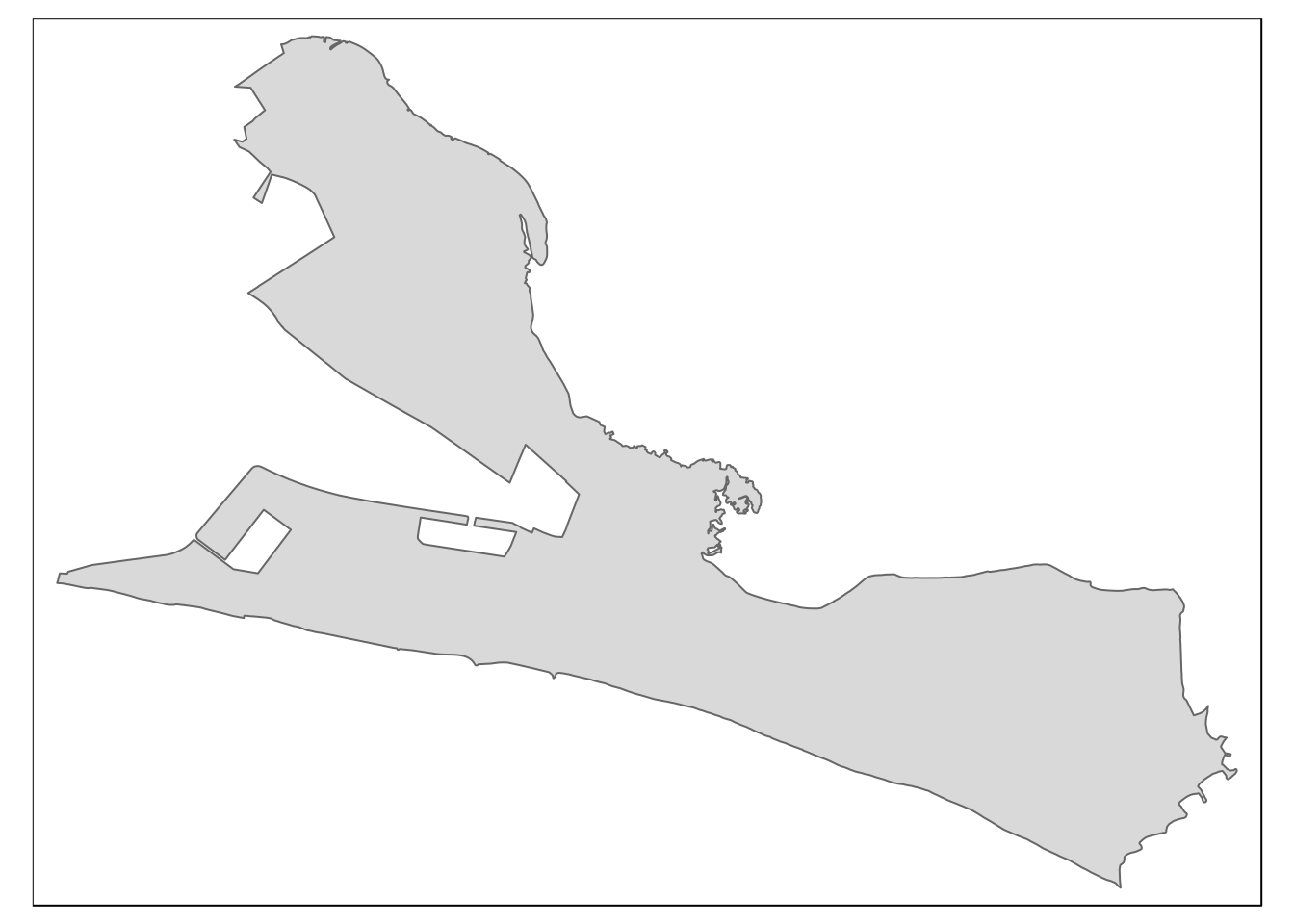

hh_habitat<-sprintf("select main_habit mhabitat, 
s1habtype,s2habtype,s3habtype habitat,
st_intersection(h.geom,s.geom) geom from 
(%s) s,
ph_v2_1 h 
where st_intersects(h.geom,s.geom)",hh_query)

habitats<-st_read(conn, query=hh_habitat)
qtm(habitats, "mhabitat") +tm_style("classic")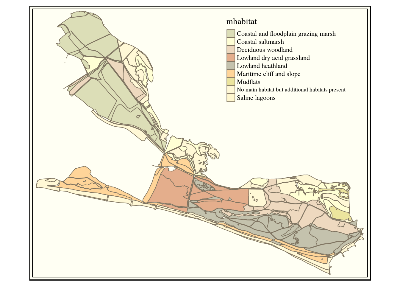

The query below extracts the paths.

hh_paths<-sprintf("select st_intersection(way,geom) geom from  (%s) s,
dorset_line l where st_intersects(way,geom)", hh_query)

paths<-st_read(conn, query=hh_paths)
qtm(paths)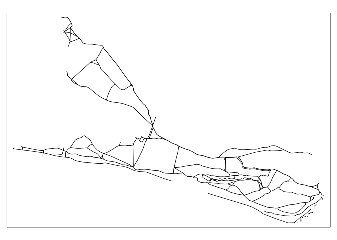

Now to reproduce the buffering analysis for Hengistbury head we just need to drop in queries that returned results for Hengistbury head instead of those which pulled the layers from the Arne schema. The sprintf trick is invaluable again here, as typing out the full query would be very tedious and error prone. As it is, all the code has been tested for Arne and all that is needed is to place the Hengistbury select queries within brackets.

query1<-sprintf("select mhabitat,st_buffer(st_union(geom),0.1) geom 
from (%s) s group by mhabitat ",hh_habitat)

query2<-sprintf("select st_buffer(st_union(geom),50) geom 
from (%s) s",hh_paths)

query3<-sprintf("select mhabitat,st_difference(h.geom,p.geom) 
    geom from (%s) h, (%s) p",query1,query2)

dif<-st_read(conn,query=query3)

qtm(dif,"mhabitat") +tm_style("classic")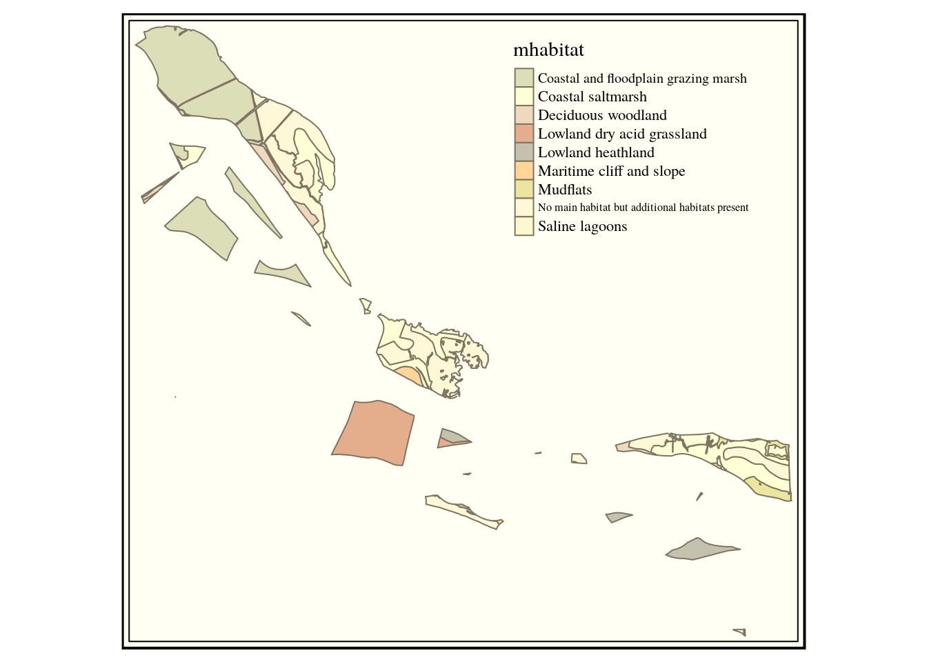

9.4.3 Exercises

We can see that there is much less undisturbed habitat of any type at Hengistbury head. This could be quantified and experiments run with different buffer widths.