Section 11 Combining raster and vector data
One of the advantages of running terrain analysis in R as shown in section 10 is that it is very easy to continue to work with the data in order to build up a more complete analysis through combining raster and vector data. One example of this is the species distribution modelling shown in section 13
In this section we’ll see how some of the operations shown in the previous sections can all be combined together to produce some useful analysis.
In a field course students counted the numbers of pines that were regenerating within randomly placed quadrats on Coombes heath at Arne.
For each quadrat the students wanted to know the distance to the paths, the slope, insolation, topographic wetness index and distance to the nearest tree.
Let’s simulate data across the Arne heathland as an exercise to demonstrate how the GIS techniques can fill in these variables.
require(RPostgreSQL)
library(giscourse)
library(mapview)
library(raster)

mapviewOptions(basemaps =c("OpenStreetMap","Esri.WorldImagery",
                           "Esri.WorldShadedRelief",
                           "Stamen.Terrain"))

conn <- connect()
11.1 Loading data
11.1.1 Loading the Arne raster data
We’ll use the data that was produced through terrain analysis. This was saved in the local file structure under /rasters/arne.It was also pushed onto the postgis data base.
slope<-raster("rasters/arne/slope.tif")
sol<-raster("rasters/arne/insol_oct.tif")
twi<-raster("rasters/arne/twi.tif")
dsm<-raster("rasters/arne/dsm.tif")
dtm<-raster("rasters/arne/dtm.tif")
If the files are not available locally they can be pulled from postgis (this takes a little bit longer to run. Use local files if they are available
# dsm<-pgGetRast(conn,c("arne","dsm"))
# dtm<-pgGetRast(conn,c("arne","dtm"))
# slope<-pgGetRast(conn,c("arne","slope"))
# sol<-pgGetRast(conn,c("arne","insol_oct"))
# twi<-pgGetRast(conn,c("arne","twi"))
11.1.1.1 Vector data
Let’s just work on the areas of heathland at the Arne reserve. The following queries should now be understandable. The first query extracts all the heathland and combines it into a geometry. The areas of heath are buffered by 10m, as the original polygons are split by paths. We neither want nor need these splits. The second query extracts only the paths that fall within the heathland
## subquery for heath
query1<- "select * from arne.phabitat where mhabitat ilike '%heath%'"

## Drop it into the query shown in the geoprocessing section

heath_sql<-sprintf("select mhabitat,st_buffer(st_union(geom),10) geom
from (%s) a group by mhabitat",query1)

heath<-st_read(conn,query=heath_sql)

query<-sprintf("select st_intersection(p.geom,h.geom) geom
from arne.paths p, (%s) h where st_intersects(p.geom,h.geom) ",heath_sql)
paths<-st_read(conn,query=query)
There is also a study area polygon that was digitised in QGIS and loaded into the arne schema.
study<-st_read("rasters/arne/study_area.shp")
#> Reading layer `study_area' from data source `/home/rstudio/webpages/books/GIS_course/rasters/arne/study_area.shp' using driver `ESRI Shapefile'
#> Simple feature collection with 1 feature and 1 field
#> geometry type:  POLYGON
#> dimension:      XY
#> bbox:           xmin: 396463.7 ymin: 86716.44 xmax: 398051.4 ymax: 87905.42
#> epsg (SRID):    NA
#> proj4string:    +proj=tmerc +lat_0=49 +lon_0=-2 +k=0.9996012717 +x_0=400000 +y_0=-100000 +ellps=airy +units=m +no_defs
st_crs(study)<-st_crs(heath)
st_write(study,conn,c("arne","study_site"),overwrite=TRUE)study<-st_read(conn,query="select * from arne.study_site") So we can take the difference between the layers
paths<-st_intersection(paths,study)
heath<-st_intersection(heath,study)
Check the data visually
map<-mapview(heath) +mapview(paths)
map
11.1.2 Producing a canopy height model
This can be achieved using a simple bit of map algebra. The canopy height is the difference between the dsm and dtm. Sometimes this produces a slight negative reslt, which are errors. These can be set to zero
chm<-dsm-dtm
chm[chm<0]<-0
chm<-raster::crop(chm,as(heath,"Spatial"))
The chm can be masked to the heathland
chm<- raster::mask(chm,heath)
plot(chm)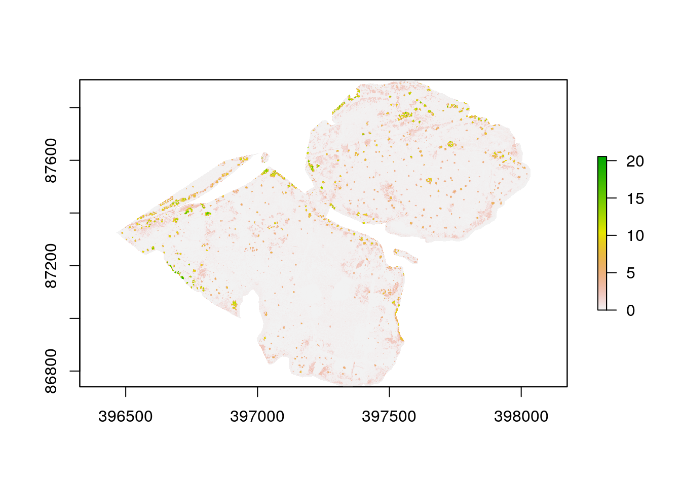
11.1.3 Simulating quadrats
Let’s simulate data from 200 quadrats placed randomly within the heath geometry.
quadrats <- st_sample(heath, size=200, type='random')
st_crs(quadrats)
#> Coordinate Reference System:
#>   EPSG: 27700
#>   proj4string: "+proj=tmerc +lat_0=49 +lon_0=-2 +k=0.9996012717 +x_0=400000 +y_0=-100000 +ellps=airy +towgs84=446.448,-125.157,542.06,0.15,0.247,0.842,-20.489 +units=m +no_defs"
11.1.3.1 Extracting values
Extracting all the raster values for the quadrats is simple. The easiest approach is to form a stack of all the raster layers. The data is the extracted for each point as a data frame. The quadrat points have to be coerced to the older spatial class. This just involves using as(quadrats,“Spatial”)
stk<-raster::stack(slope,sol,twi,dsm,dtm)
df<-data.frame(raster::extract(stk,as(quadrats,"Spatial")))
head(df)
#>        slope insol_oct      twi    dsm    dtm
#> 1  3.3668809  1.639939 3.141956  5.353  5.185
#> 2  1.5124466  1.671114 4.827164 14.170  6.190
#> 3  1.0087041  1.897353 4.365872  4.665  4.573
#> 4  0.5661839  1.789227 4.335808 12.858 12.830
#> 5  5.4394178  1.762317 2.194184  3.990  3.875
#> 6 12.5716362  2.474135 2.014426  4.843  4.840
What if we want mean values around the quadrats? That might be a better measure when taking into account slope than the slope at 2m resolution. In other words topography, rather than micro topography. There are two approaches to this. One is to coarsen the resolution of the raster itself then run the overlay as usual. This is probably the best approach and introduces the useful concept of raster aggregation. There are many reasons to aggregate rasters to a coarser resolution by applying a statistic. Quicker methods of coarsening a raster tend to simply use the nearest neighbour to the centre of the new grid, which may not be what we want in many cases.
slope_5 <-aggregate(slope, fact=5, fun=mean, expand=TRUE, na.rm=TRUE)
df$slope_5 <-raster::extract(slope_5, as(quadrats,"Spatial"))
The other approach is to buffer around the points when extracting. The two methods should produce very similar results, although the first is based on squares and the second circles.
df$slope_5 <-raster::extract(slope_5, fun=mean,as(quadrats,"Spatial"),buffer=5)quadrats<-st_bind_cols(df, quadrats)
plot(quadrats)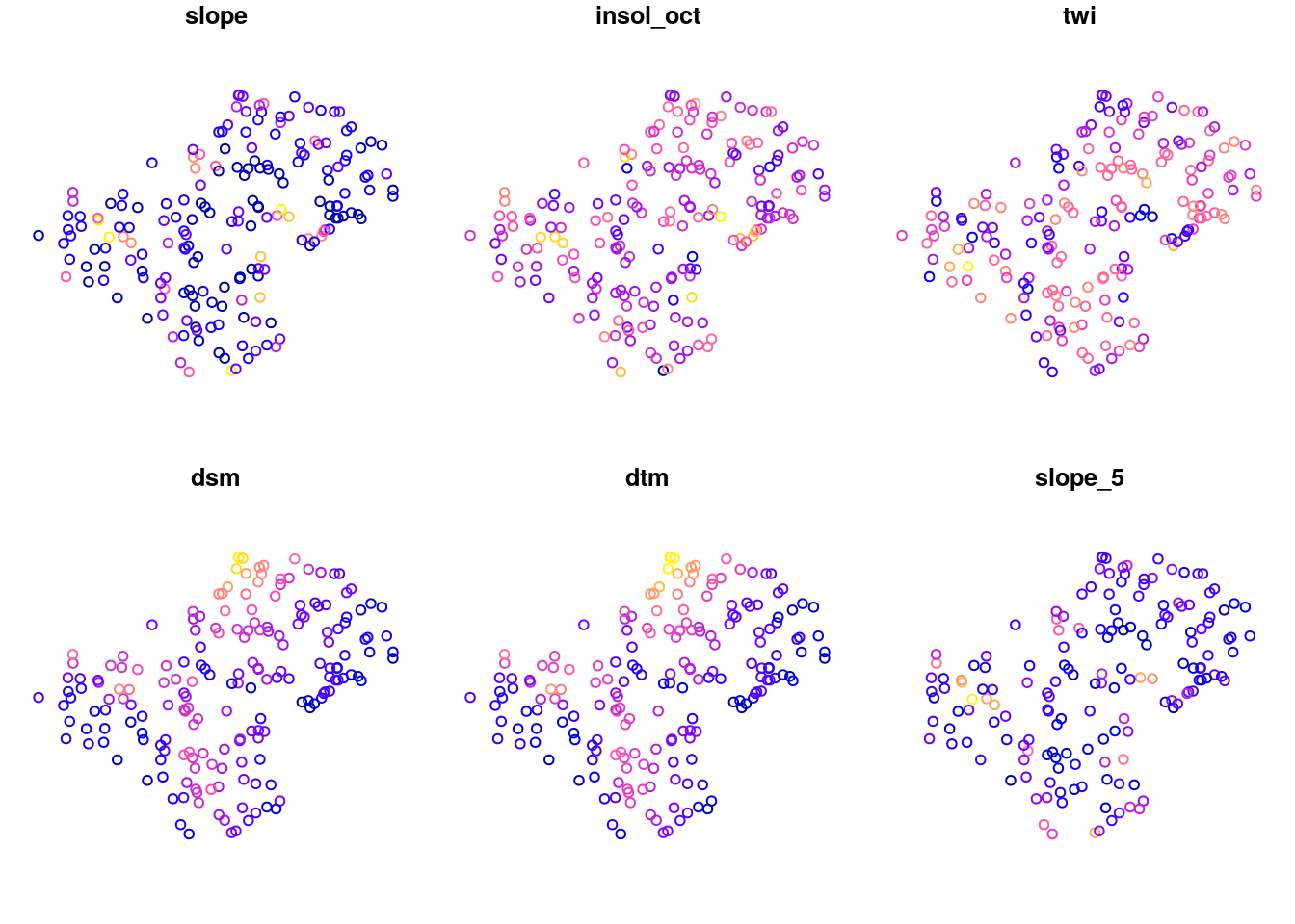
11.2 Finding the trees
Distances are measured between objects. So most of the time we need to vectorise raster layers in order to measure distances. There are exceptions to this, and raster layers are very important elements when calculating least cost paths, as they provide input as cost surfaces. However in this case the simplest way to find the distance from a quadrat to a tree is to produce a layer of vectorised “trees” from the canopy height model. Providing there are no buildings and other objects that could be classified as trees this involves two steps.
- Raster algebra to define two classes of vegetation (high and low)
- Vectorisation of the classes.
This is achieved with the code below.
chm[chm<2]<-NA ## Set below 2m as blanks (NA)
chm[chm>=2]<-1 ## Set above 2m to a single value
trees<-rasterToPolygons(chm, dissolve=TRUE)
trees<-st_as_sf(trees)
st_crs(trees)<-st_crs(heath)
mapview(trees)
11.2.0.1 Forming a distance matrix
The distance matrix contains every combination of quadrat and tree. Take care to check the dimensions before forming distance matrices in this rather “brute force” manner, as they could run out of memory. In this case there is no problem. In fact the st_distance function in R is extremely well designed to avoid problems with memory as it uses sparse matrices and lazy evaluation. This is benefit of the Red Queen effect. A few years ago it would have been a computational challenge to form the distance matrix. Not any more.
# Cast trees to single polygons.
# Note that if we didn't do this we would just get the nearest neighbour distances, which may be a good thing in some cases.
trees<-st_cast(trees$geometry,"POLYGON")

distances<-st_distance(quadrats,trees)
dim(distances)
#> [1]  191 1569
Now, one we have all possible distances, all we need to do is to calculate the minimum to know how far each quadrat is from a tree.
quadrats$min_dist<-apply(distances,1,min)We can do other operations in the same way. For example. how many trees are within 100 meters. Really easy. Just make a function and apply it to the matrix.
f<-function(x) sum(x<50)
quadrats$n50<-apply(distances,1,f)
Now we can check that its all gone to plan by visualising the result as a mapview. Clicking on the points gives the values and if there is any doubt, adding the leaflet extras gives a measuring too.
mapview(quadrats,zcol="min_dist") +mapview(trees) -> map
map %>% extras()
11.2.1 Exercises
Calculate the distance between the quadrats and the paths and add this measure to the data frame.
rm(list=ls())
lapply(paste('package:',names(sessionInfo()$otherPkgs),sep=""),detach,character.only=TRUE,unload=TRUE)