Section 5 Coordinate reference systems

5.1 Concepts

The use of a coordinate reference systems distinguishes a GIS from software used for processing images such as photographs. Although both raster data and vector data can be drawn on the screen without reference to the surface of the planet, this would not be useful in the context of a Geographical study. The coordinate reference system links the coordinates held in the data source with the surface of the Earth. If coordinates are in latitude and longitude they are referenced to the equator and the Greenwich Meridian. The units are degrees, which are not useful measures of either area nor distance

Geographical coordinates require projection in order to be used for measurement. The units for the coordinates in the British National grid CRS are meters, as this is a projected CRS. However there is no obvious origin for this CRS when seen from a global perspective. The location of National Grid’s nominal origin , in the sea off Cornwall, ensures that most locations in the UK have positive Easting and Northing values. In fact the true origin (datum) for the projection is in the middle of the country at 2° W and 49° N in order to keep distortion to a minimal. The British national grid is a strictly local CRS that is used in the UK, but not elsewhere. See figure 5.1

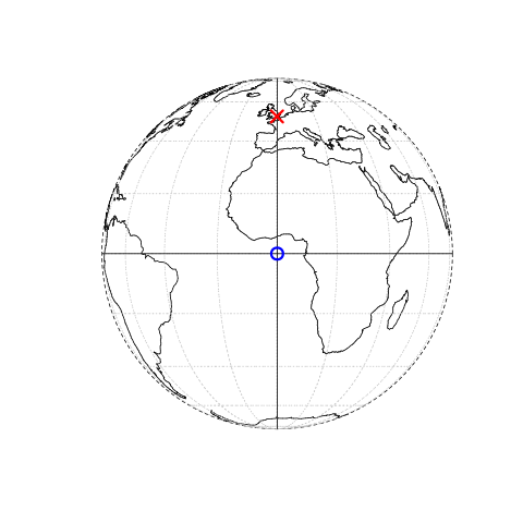
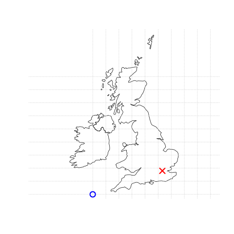
Contrasting Geographical coordinates (EPSG 4326) with British National Grid (EPSG 27700). The left plot has its origin at 0° longitude and latitude. The Bristsh national grid has an origin located in the sea west of Cornwall (Figure from https://geocompr.robinlovelace.net/).

Figure 5.1: Contrasting Geographical coordinates (EPSG 4326) with British National Grid (EPSG 27700). The left plot has its origin at 0° longitude and latitude. The Bristsh national grid has an origin located in the sea west of Cornwall (Figure from https://geocompr.robinlovelace.net/).

It is very important to know which CRS you are using and to be aware of which CRS is used by the data. The issue can become complicated when working with data provided by researchers in more than one country. Each nation may use a different gridded system for projection. The datums used for the projections may also have changed over time. To help enforce consistency the European Petroleum Survey Group (EPSG) catalogued all the known CRSs in use and provided them with a common code number for reference. The EPSG code is the simplest and most consistent way to refer to a CRS.

In the UK there are three very commonly used EPSG codes.

EPSG 4326: This is the code for unprojected (i.e. Latitude and Longitude) geographical coordinates. It is universal and global in extent. This is the best CRS for raw data as all the others can be easily derived from it, no matter where you are.
EPSG 27700: The British National grid. The default national system that respects distances and areas. This is the CRS for site mapping in the UK.
EPSG 3857: Web Mercator. The projection used by Google maps and many other online sources.

All GIS can reproject data from latitude and longitude form into a projection for calculating distances and areas it is generally preferable to keep data that may be shared internationally in EPSG 4326. When working with researchers in the UK the British national grid, EPSG 27700 is very commonly used as the standard format and most data will be provided in this CRS.

EPSG 3857 is convenient for global visualisation of web maps. However the calculations made directly within this CRS are rather inaccurate and it is preferable to use EPSG 27700 when working on projected data in the UK.

5.2 QGIS: Projection

QGIS now has excellent on the fly re-projection capability. On the fly re projection is an extremely useful feature of a desktop GIS. However it is also a feature that must be treated carefully.

Be very careful with on the fly reprojection. You must remember that the coordinates of a layer that is being reprojected will not have changed on the file nor in the data base. Although layers will all line up visually, if two layers are actually held in different coordinate reference systems then any geocomputation ivolving both layers will not work!.

5.2.1 Checking the CRS of each layer

Due to the potential pitfalls of on the fly re-projection, you should always check that you know the actual CRS of the layers that you are using in a desktop GIS project. Do not take the CRS for granted when working at multiple scales (e.g global and UK). You can check by looking at the information for each loaded layer. So, for example, figure 5.2 is showing the natural earth low resolution countries layer that has been loaded into QGIS from the postgis data base used on this course. This is a global layer, so it is unprojected (i.e. in EPSG 4326). Hovering on the layer name provides basic information and right clicking the layer brings up the properties menu.

Figure 5.2: Finding the CRS of the data file in QGIS. Hovering over the name in the layers panel provides a popup with this information. Right clicking the name of the layer to bring up the properties gives more information. Always check that you know the true CRS of every data source.

5.2.2 Reprojecting on the fly

Re-projection on the fly in QGIS is conducted by setting the project level CRS. This can be done by clicking in the bottom right hand corner and searching for an appropriate CRS in the menu see figure 5.3 for an animation of the procedure. Re-projection on the fly will change the appearance of all the loaded maps, but it does not change the underlying data. Re projecting the world into British national grid clearly makes no sense, but it can be done, as shown by figure 5.3.

Figure 5.3: Projecting a world map into British National grid: This is not a good idea. The projection is not appropriate for the global data!

Re-projection from EPSG 4326 at the appropriate UK scale will work just as expected. This is shown in figure 5.4.

Figure 5.4: Changing between EPSG 4326 and EPSG 27700

If you load base maps from the xyz tiles menu the maps will also be projected from the native EPSG:3857 web Mercator into British national grid. See figure 5.5.

Figure 5.5: Changing between EPSG 4326 and EPSG 27700

5.2.3 Reprojecting the layer itself

In order to permanently change the projection of a layer itself in QGIS you need to form a new file. This step is required, as re-projection on the fly has not actually altered the stored coordinates. Figure 5.6 shows the steps.

Saving a layer in a new projection. In this case the simpler outline of the UK was held in the postgis data base in EPSG 4326. Saving the file into British national grid reprojects the coordinates. Right click on the file name in the layers panel. Choose the projection and file name. Adjust the extent if necessary.

Figure 5.6: Saving a layer in a new projection. In this case the simpler outline of the UK was held in the postgis data base in EPSG 4326. Saving the file into British national grid reprojects the coordinates. Right click on the file name in the layers panel. Choose the projection and file name. Adjust the extent if necessary.

Notice that the project CRS is set to EPSG 4326 throughout this example This does not change, so although the new layer is being reprojected into British National Grid it will still look as if the layer is in EPSG 4326. It is simply being reprojected on the fly again to keep the visual presentation consistent. This is why on the fly reprojection can easily cause confusion, if you are not careful. Always check the CRS!

In the example above the file was clipped to the map extent when saving. When building up site specific analyses in QGIS you will often save elements of larger coverages in order to form a local project for analysis. This is shown in more detail in section 7

A final warning. Because introductory classes in GIS typically provide data in a common CRS the problems that can arise when CRSs are mixed are frequently overlooked. It is very important to be aware that spatial operations on data in mixed CRSs are simply not possible. Even though the maps may appear to be loaded in the same project as a result of on the fly reprojection, they may not be lined up. Ignore this warning at your peril!

5.3 R: Coordinate reference systems

require(giscourse)
require(tmap)
conn <- connect()

5.3.1 Finding the CRS

The simple features library is designed to be compatible with postgis. Many of the functions have the same names as the operators used in spatial sql.

Let’s load a simple world layer from the natural earth package in R.

require(rnaturalearth)
countries<-ne_countries(returnclass = c("sf"))

To find the CRS of the layer we type

st_crs(countries)
#> Coordinate Reference System:
#>   EPSG: 4326 
#>   proj4string: "+proj=longlat +datum=WGS84 +no_defs"

Notice that the information on the CRS is provided in two formats. The first is the EPSG code. The second is the proj4string. The second seems rather cryptic. The technical details are that R uses an open source library of re-projection code called proj4 (so does QGIS, although this is less explicit). The proj4string contains a list of options that proj4 understands for re-projection.

Usually it is only necessary to remember the EPSG code to re project. In figure 5.7 the world layer is shown unprojected

qtm(countries) +tm_grid() + tm_style("natural")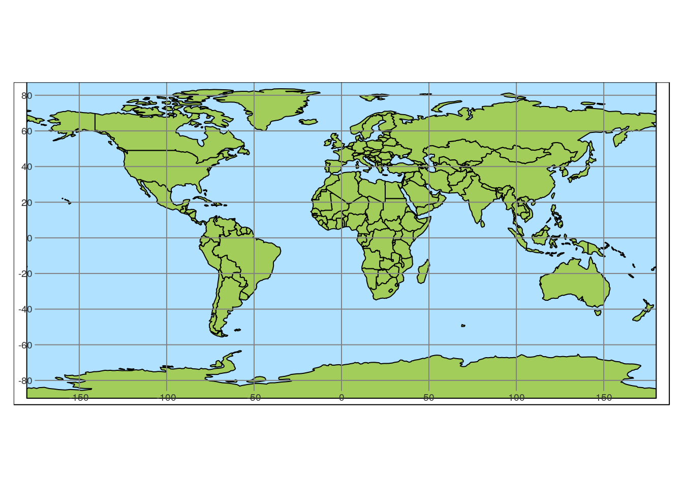

Figure 5.7: Natural earth countries layer unprojected (EPSG:4326)

5.3.2 Global projections using proj4

To quickly re project global data sets to a wide range of projections look at the proj4 web site

https://proj4.org/operations/projections

For example in figure 5.8 the world layer is re-projected to Goode Homolosine using the proj4string shown on the page

https://proj4.org/operations/projections/goode.html

proj<-"+proj=goode"
coun<-st_transform(countries,proj)
qtm(coun) +tm_grid() + tm_style("natural")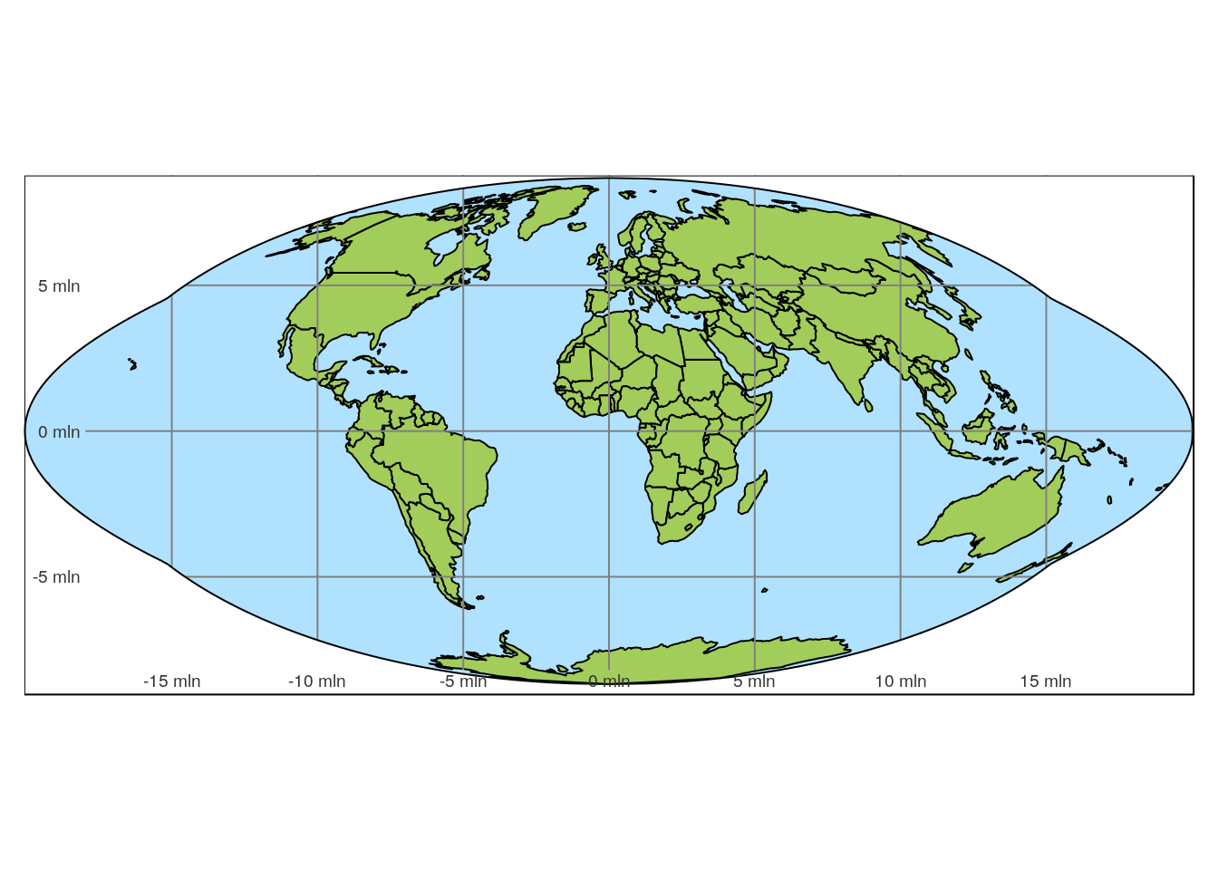

Figure 5.8: Countries of the world projected to the Goode Homolosine projection

proj<-"+proj=robin"
coun<-st_transform(countries,proj)
qtm(coun) +tm_grid() + tm_style("natural")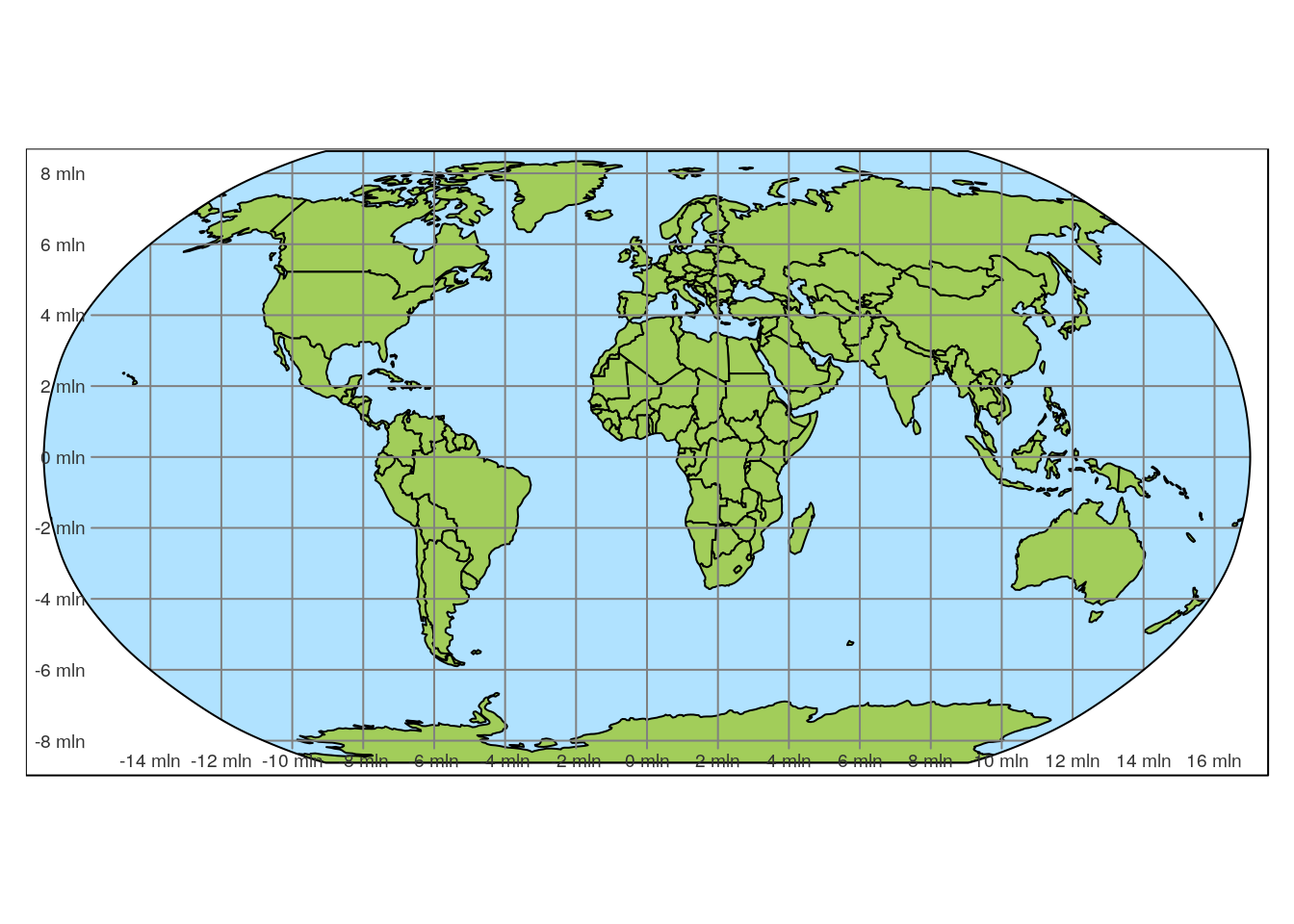

Figure 5.9: Countries of the world projected to the Robinson projection

5.3.3 Checking the coordinate reference system used in postgis

Piping a single geometry into st_crs is a quick way of finding the crs in postgis from R

st_read(conn, query ="select geometry from gbif limit 1") %>% st_crs() 
#> Coordinate Reference System:
#>   EPSG: 4326 
#>   proj4string: "+proj=longlat +datum=WGS84 +no_defs"
st_read(conn, query ="select geom from counties limit 1") %>% st_crs() 
#> Coordinate Reference System:
#>   EPSG: 27700 
#>   proj4string: "+proj=tmerc +lat_0=49 +lon_0=-2 +k=0.9996012717 +x_0=400000 +y_0=-100000 +ellps=airy +towgs84=446.448,-125.157,542.06,0.15,0.247,0.842,-20.489 +units=m +no_defs"
st_read(conn, query ="select geometry from waterways limit 1") %>% st_crs()  
#> Coordinate Reference System:
#>   EPSG: 27700 
#>   proj4string: "+proj=tmerc +lat_0=49 +lon_0=-2 +k=0.9996012717 +x_0=400000 +y_0=-100000 +ellps=airy +towgs84=446.448,-125.157,542.06,0.15,0.247,0.842,-20.489 +units=m +no_defs"

5.3.4 Transforming

St_transform will work either in postgis or in R.


require(dplyr)
ne_countries(scale = 10, returnclass = "sf") %>% filter(name=='United Kingdom') ->uk
st_crs(uk)
#> Coordinate Reference System:
#>   EPSG: 4326 
#>   proj4string: "+proj=longlat +datum=WGS84 +no_defs"

uk_27700<-st_transform(uk,27700)

t1<-tm_shape(uk) + tm_fill() + tm_borders()   +tm_grid() + tm_style("classic")
t2<-tm_shape(uk_27700) + tm_fill() + tm_borders()   +tm_grid() + tm_style("classic") 
tmap_arrange(t1,t2)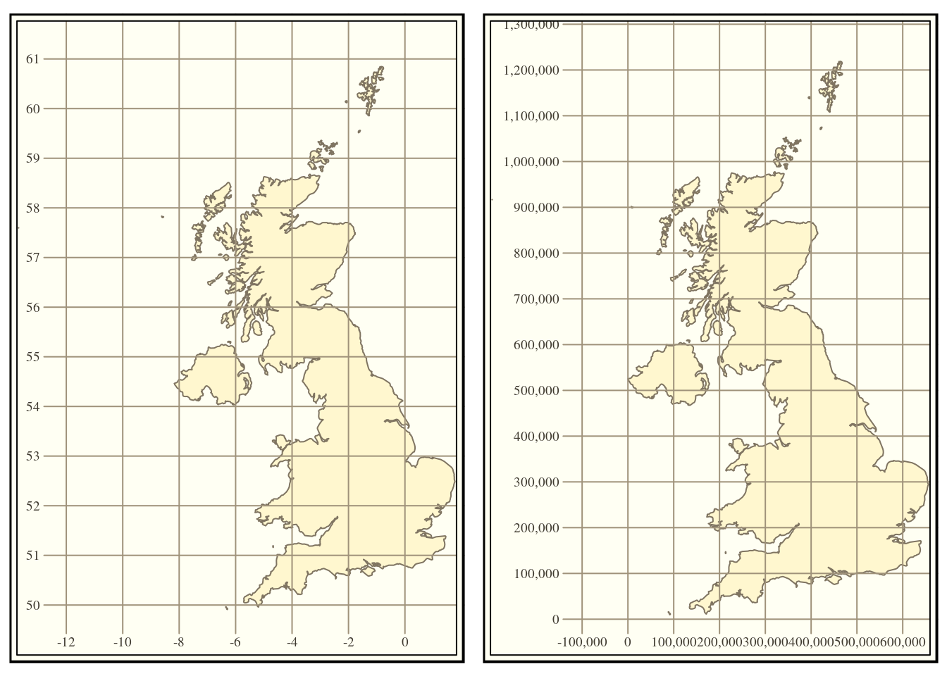

UK displayed using the qtm function in R in unprojectd (EPSG 4326) form and in British National gid (EPSG 27700). Note that because the map making package aims to keep the aspect ratio constant the maps look very similar, apart from the grid coordinate values.

Figure 5.10: UK displayed using the qtm function in R in unprojectd (EPSG 4326) form and in British National gid (EPSG 27700). Note that because the map making package aims to keep the aspect ratio constant the maps look very similar, apart from the grid coordinate values.

5.3.4.1 Transforming in postgis

This is a slightly more complex postgis query that uses some of the concepts in later sections. Notice that layers such as natural earth are held in EPSG 4326. If an outline of the UK was derived within the data base from this layer it would not match up with layers held in British national grid. However it is easy to fix this my transforming in postgis itself.

query<-"select st_transform(geometry,27700) geom, name from nat_earth_countries_hi where name = 'United Kingdom'"
st_read(conn,query=query) %>% qtm() +tm_grid() + tm_style("classic")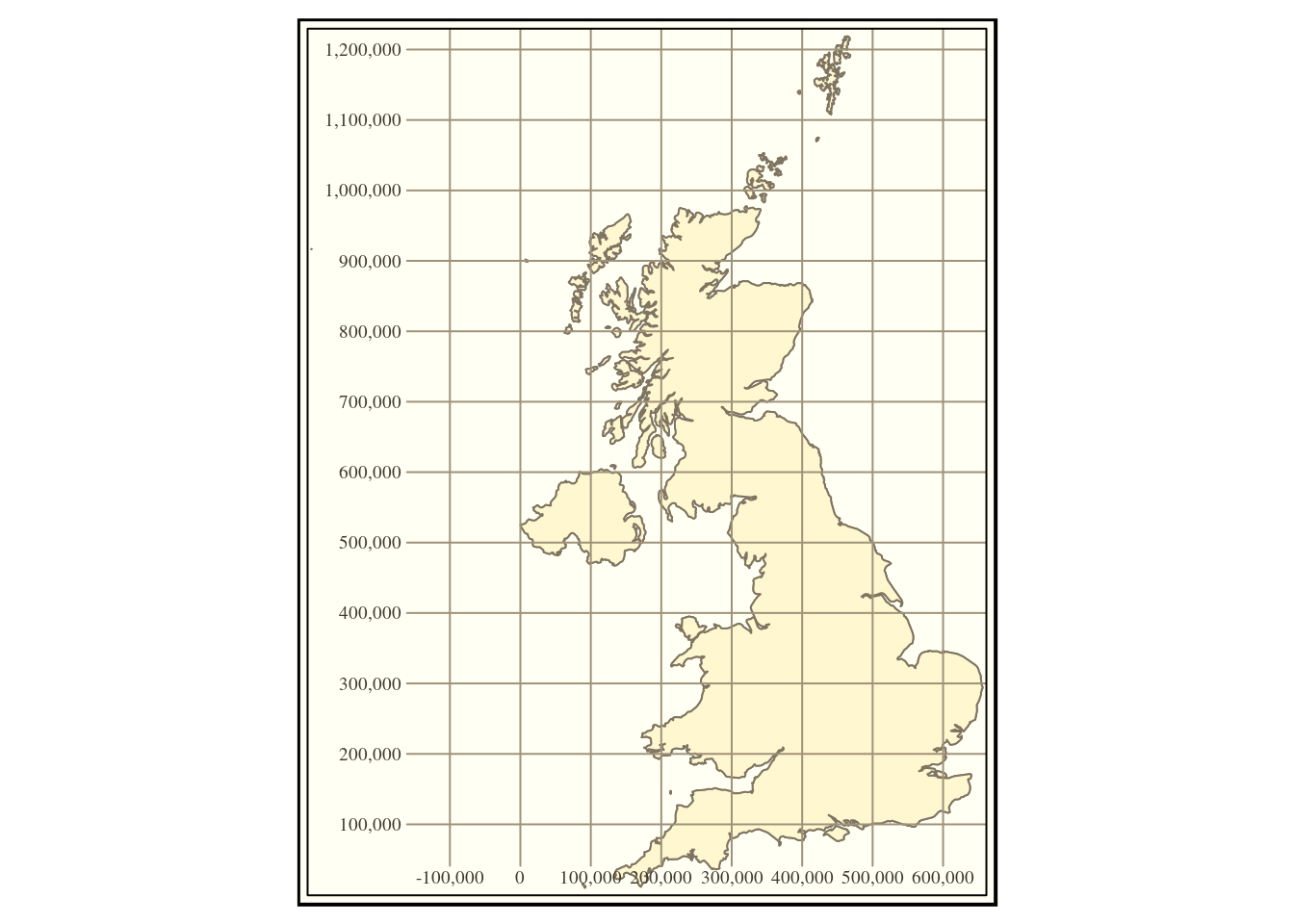

5.3.5 On the fly reprojection with mapview

The “on the fly” concept that we saw in QGIS doe not really apply in R, as most of the operations are explicitly on the data in memory. If two objects that are involved in a spatial operation are in different CRSs then R will throw an error message.

The mapview package for interactive web mapping now does include a spatial transform in the code that effectively works like on the fly re-projection. So if we view polygons of the UK in EPSG 4326 and EPSG 27700 in the same mapview they appear identical.

mapview(uk_27700) +mapview(uk)