Section 6 Attribute queries
6.1 Concepts
6.1.1 Selecting subsets of data
A very common element of GIS is the selection of subsets of a larger data set for analysis. There are many reasons for this. We may be interested in the distribution of a single species and want to find only the occurrences of this particular species from a record set that includes multiple species. There are many approaches to narrowing a data set. Very often data are available online from a source which provides the filtering tools. As an example of this, the gbif function in the R package dismo uses the search engine provided by the gbif occurrence API https://www.gbif.org/developer/occurrence.
# require(dismo)
# d<-gbif("Polyommatus","coridon",geo=TRUE) # get all records of Chalkhill blues from GBIF
When the line above is run in R a huge online data base is being filtered in the “cloud” in order to select records for a given genus and species. However this often leads to a significant download time. It took over an hour to fetch all records of the chalkhill blue butterfly. An online filter would not be run more than once when studying a species or group of species. The table “blues” in the postgis data base has been produced by downloading all the records of adonis and chalkhill blue butterflies from gbif.
The data could be recreated and updated by fetching the records again but this action would need to be taken at the start of each analysis, which would be slow. So it has been placed in the local networked data base for speed. See section 13.2.1.1.
Often a study focusses on a particular site, or group of sites. Sometimes a particular habitat type is the focus. So in order to begin many GIS based analysis we frequently first need to narrow down the available data in some respect.
6.1.2 Working with single large tables in PostGIS
One of the key advantages of including a spatial data base in a GIS project is that it makes all the data management fully scaleable. A well designed data base can hold anything from tens to millions of observations of the same type of features without making any changes to the underlying structure. A correctly designed data base, with correctly indexed fields, can process 10 million observations in just a few seconds.
For example, the table ph_v2_1 in the gis_course data base holds over half a million polygons. These represent all the recognised priority habitat patches across the whole of the South of England. This table is actually a subset of a larger data set of priority habitats in England and Wales. The subsetting was conducted by the data providers in order to reduce the size of the files when downloading them from their web site. However, there is no intrinsic reason to split this dataset up in this way. As each of the files of priority habitats has identical attributes they could all be placed in a single table within a spatial data base. The table would then be indexed, which speeds up searching within the table make it a matter of seconds. So, the ph_v2_1 files for the midlands and north of england could be added to the contents of the table in order to produce a single national data file of priority habitats. This table would be over 30 GB in size, so it could not be opened directly as a shapefile. However when held in a postgis data base there are no problems searching for records within it. Keeping data together in single, indexed and searchable tables allows analyses to be designed that could be run for any of the millions of priority habitat sites in the UK without beginning from scratch.
When working on your own GIS projects there are two approaches to filtering data. The simple approach is to just load a whole vector layer from a shapefile or from a postgis table and then filter the parts you wish to use using techniques within the desktop GIS. This works very well, providing the data is not too large to fit into memory and/or to slow down rendering of layers on the desktop GIS. However it would not work for the ph_v2_i table.
A more scaleable solution is to write an SQL query that only pulls in the parts of the table that are needed from the large tables held in the data base itself. This is the only approach that will work with really large data sets held in the data base and does involve learning some simple sql.
6.2 QGIS
In order to run an sql query in postgis from QGIS we use the db manager. You can use this tool to browse the data tables as shown in section 4.3.
The process of running an SQL query involves carefully constructing a syntactically correct statement that filters out the rows that match to a where clause.
Let’s try a realistic example. We will select all the calcareous grassland from the priority habitat (ph_v2_1) layer. There are both highland and lowland grassland types. We want to find matches to either.
SQL (structured query language) can be quite difficult to write and understand. However this particular form of SQL query is reasonably simple in form. It reads almost like an English sentence. There are only two parts to it. The query reads
select * from ph_v2_1 where main_habit ilike ‘%calc%grass%’
First we want to select all the columns.So the query begins with
select * from ph_v2_1
Note that the asterix stands for everything, i.e. all the columns.
We then just need a clause which filters the rows. So the second part of the query looks for matches to a condition.
where main_habit ilike ‘%calc%grass%’
This is a bit more complicated. By using ilike we are filtering on an approximate match. The query looks for any characters before calc then a gap then grass then a gap. This returns all the calcareous grassland whether the words lowland or highland are also included in the text.
Watch figure 6.1 to see the way QGIS helps you to type in the query. As you type in the sql window you will see helpful prompts appear that suggest the names of the tables you can include and the syntax of the query. This doesn’t completely automate the process, as you must still understand the rules of sql to effectively form a query. However it does make it easier to choose the elements. Figure 6.1 shows the process of writing this query in action. Notic how the prompts are offered by the interface.
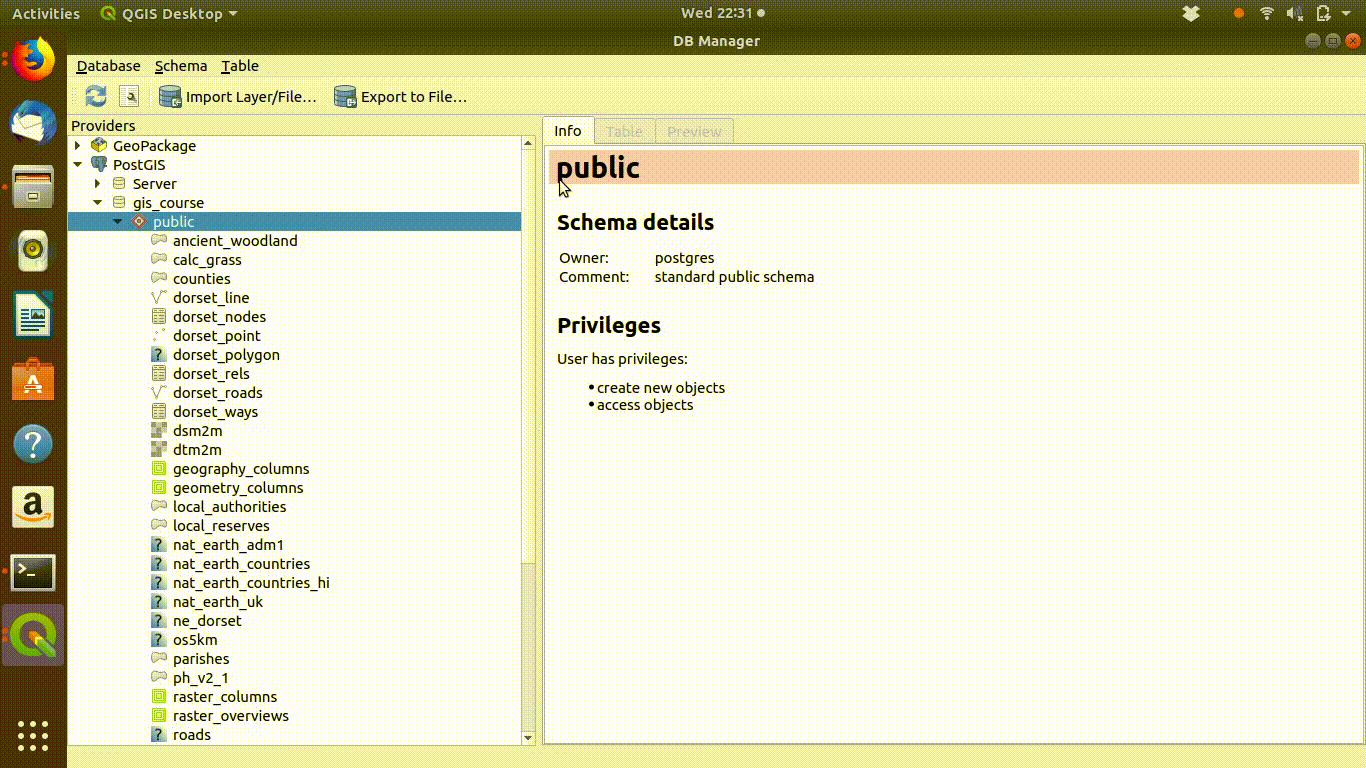
Figure 6.1: Forming a simple query in the QGIS DB manager. The query text is select * from ph_v2_1 where main_habit ilike ‘%calc%grass%’. Prompts appear at each stage as the text is typed in. This makes it easier to select tables and field names.
Once the query has run through the result can then be added to the project. Figure 6.2 shows this. In this case the query is realistically large. It takes some time to run, but results in a useful reduction of the very large initial data layer.
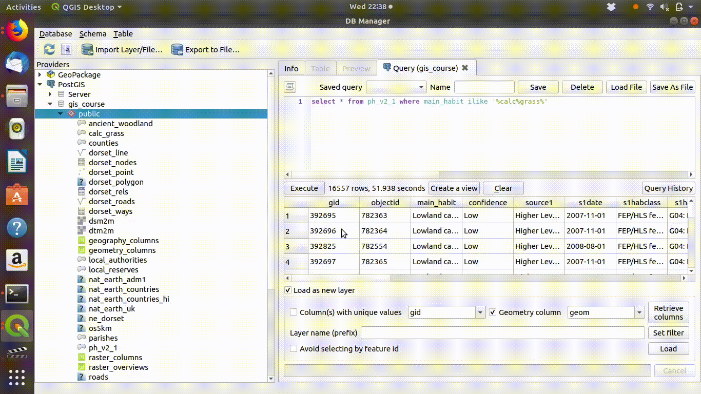
Figure 6.2: Loading the results of the query into the QGIS canvas. The query must contain a geometry field and a unique id field in order to be loaded.
6.2.1 Querying on attributes of loaded layers
SQL can also be used on layers that are already loaded into QGIS. This is client side data processing. For example figure 6.3 shows a gridded layer of forest (note this particular layer is not in the course database and was just recorded as an example)
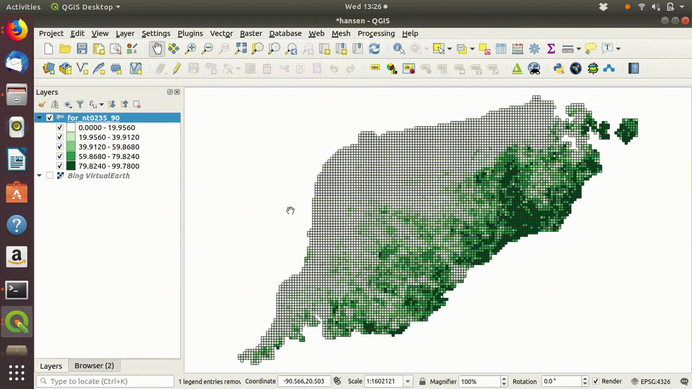
Figure 6.3: Filtering a layer that has been added to the QGIS canvas. Right click the layer and go to properties to find the sql editor. In this case grids containing forest are filtered to show a subset with forest cover over 50%
6.3 R: Querying attributes
As SQL is the language used by the database implementing queries in R is identical to implementing queries in QGIS. However unlike the db manager in QGIS no prompts are provided for writing sql in R. So, at least at the start, it can be a good idea to test a query in Qgis db manager first, then copy the query into an R script when you are quite sure that it is working as expected.
library(giscourse)
require(dplyr)
require(tmap)
conn<-connect()
6.3.1 Listing the tables in R
To find a complete searchable list of table names that can be used when working directly from R I run the following line to form an HTML table within the markdown.
dbListTables(conn) %>% as.data.frame() %>% DT::datatable()6.3.2 Example: Selecting the United Kingdom from a table of countries
The where clause in an sql statement can take many forms. For a categorical variables made up of text strings using “ilike” is quite convenient, as it is more flexible than other alternatives. Any query that works in R will also work in QGIS and vice versa. As a simple example we can extract the United Kingdom from the natural earth higher resolution countries table.
uk<-st_read(conn,query="select * from nat_earth_countries_hi where name ilike 'United%Kin%'")
#> type is 19
Let’s just test that this is what we expected.
tm_shape(uk) + tm_borders()  +
  tm_fill()  +tm_grid() + tm_style("classic") +
tm_compass(pos=c("left", "bottom")) 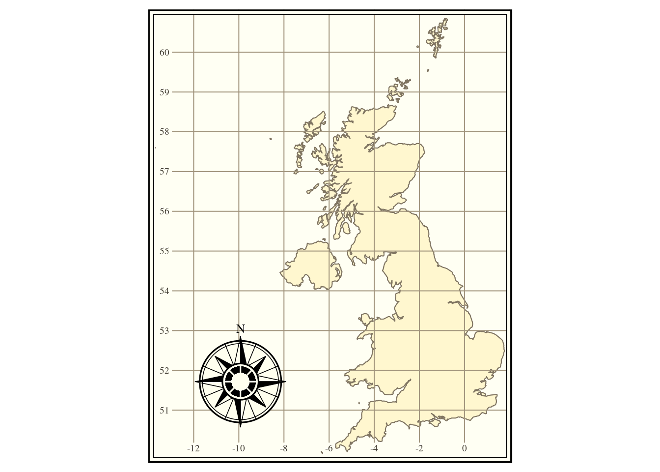
6.3.3 Another example
asia<-st_read(conn,query="select * from world where continent = 'Asia'")

tm_shape(asia) + tm_borders()  +
  tm_fill('name',legend.show = FALSE)  +
  tm_grid() + tm_style("classic") +
  tm_compass(pos=c("left", "bottom"))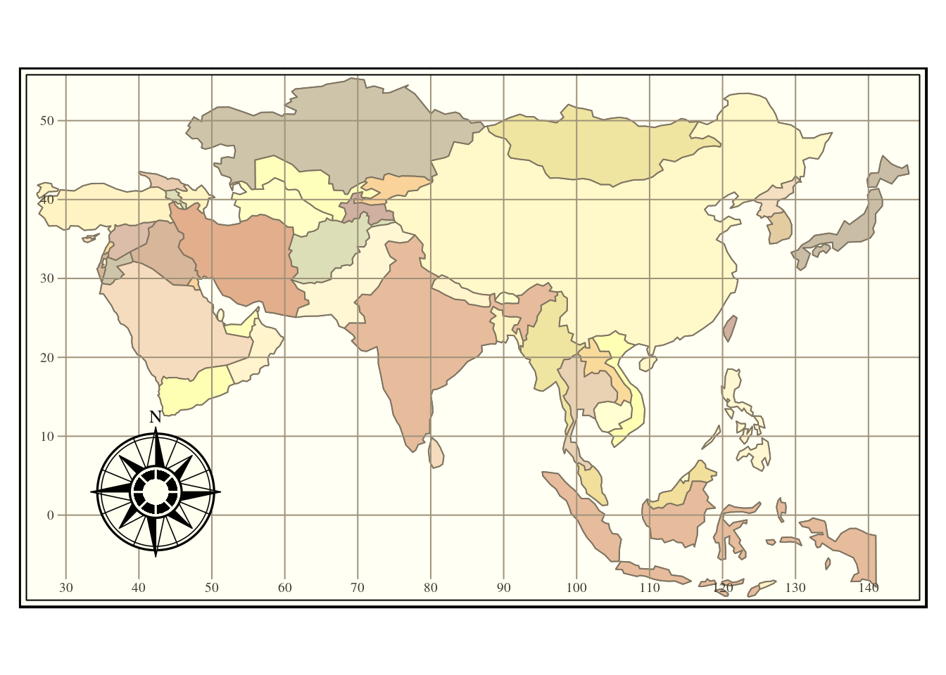
Figure 6.4: Filtering out the continent ofAsia from the natural earth countries layer.
6.3.4 More specific queries
Sometimes using ilike returns too many results. in this case it is better to be specific. For example, if we want to find the sssi for Arne RSPB reserve from the sssi table. We might first look at the names of the used for the columns of attributes, either by inspecting the table in QGIS db manager or by listing the fields.
dbListFields(conn,"sssi") %>% as.data.frame() %>% DT::datatable()We can find all the distinct names and search through them
dbGetQuery(conn,"select distinct sssi_name from sssi") %>% as.data.frame() %>% DT::datatable()If we used ilike here we might return results for more reserves than we want.
dbGetQuery(conn,"select sssi_name from sssi where sssi_name ilike '%Arne'")
#>     sssi_name
#> 1 Lindisfarne
#> 2        Arne
#> 3        Arne
Or
dbGetQuery(conn,"select sssi_name from sssi where sssi_name ilike 'Arne%'")
#>                       sssi_name
#> 1 Arnecliff and Park Hole Woods
#> 2 Arnecliff and Park Hole Woods
#> 3                          Arne
#> 4                          Arne
However if we use like, or = in the clause i t will be very specific and only return a perfect match.
arne<- st_read(conn,query="select * from sssi where sssi_name like 'Arne'")
mapview(arne)
6.3.5 Querying numerical values
Say we wanted to find all the countries in a world table with life expectancy below 70. We can use the operators <, > or = with a numerical field as input.
dbListFields(conn,"world") %>% as.data.frame() %>% DT::datatable()
world<-st_read(conn, query ="select * from world")
query<-"select * from world where life_exp < 70"
low_life_expectancy<-st_read(conn, query =query)
tm_shape(world) + tm_borders() + tm_shape(low_life_expectancy) +
  tm_fill(col="red") +tm_borders() +
  tm_style("classic") +
  tm_text("name",size="AREA",col="black") +
  tm_xlab("Countries with life expectancy below 70 years")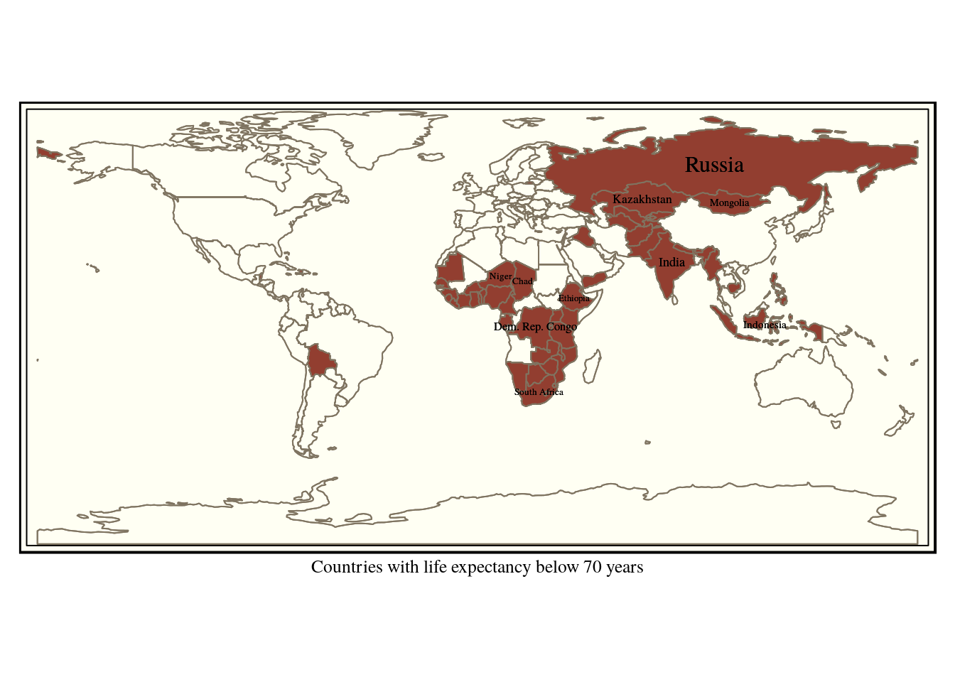
Figure 6.5: Countries with life expectancy below 70 years
6.3.6 Boolean operators
Queries can be built up to be more complex using conventional boolean logic. Say we want to find the poorest countries with the lowest life expectancy. We can look for those with a life expectancy below 70 and a gdp per capita below 1000 dollars.
query<-"select * from world where life_exp < 70 and gdp_cap_est < 1000 "
combined<-st_read(conn, query =query)

tm_shape(world) + tm_borders() +
  tm_shape(combined) +tm_fill(col="red") +
  tm_style("classic") +
  tm_xlab("Countries with life expectancy below 70 years and per capita GDP below 1000 dollars")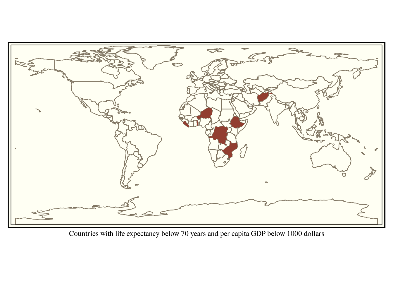
Figure 6.6: Countries with life expectancy below 70 years and per capita GDP below 1000 dollars
6.3.7 Filtering directly in R
in this particular case the world table is not in fact very large. The whole world can be held in R’s memory! This contrasts with the example of the priority habitats. So the data can be handled directly in R. There is no need to visualise all the results as maps, as the data in the sf format is just a data frame with a geometry added. For example ..
world %>% filter(continent =='Africa') %>%
  filter(life_exp > 70) %>%
  st_drop_geometry() %>%
  DT::datatable()
6.3.8 Forming tables of results in the data base
If a filtered subset of the data is going to be used many times it can be useful to form a table in the data base to hold the subset. This may speed up operations and simplify data processing. For example, if it is known that only data from Dorset is going to be of interest dorset specific tables could be formed. In the next section 7 we will see how personal schemas can be used to hold project specific data within a data base. The code that is commented out below forms a new table in “myschema”. When forming a new table it is also a good idea to add a spatial index. We want to make a table from the query
select * from ph_v2_1 where main_habit ilike ‘%calc%grass%’
# query<-"create table calc_grass as select * from ph_v2_1 where main_habit ilike '%calc%grass%'"
# dbSendQuery(conn,query) #don't need to run again
# query<- "create index spind_calc_grass on calc_grass using gist(geom)"
# dbSendQuery(conn,query)
Notice that st_simplify can be used to quickly visualise a large number of potentially complex polygons to check the result. This is a useful trick when the data set is very large. If a query returns a multi geometry with a z field (which some data contains) it needs to be wrapped in st_zm(). Remember this if you get annoying error messages.
st_zm(st_read(conn,query= "select st_simplify(geom,200) from calc_grass")) %>%
  qtm + qtm(uk,fill=NULL)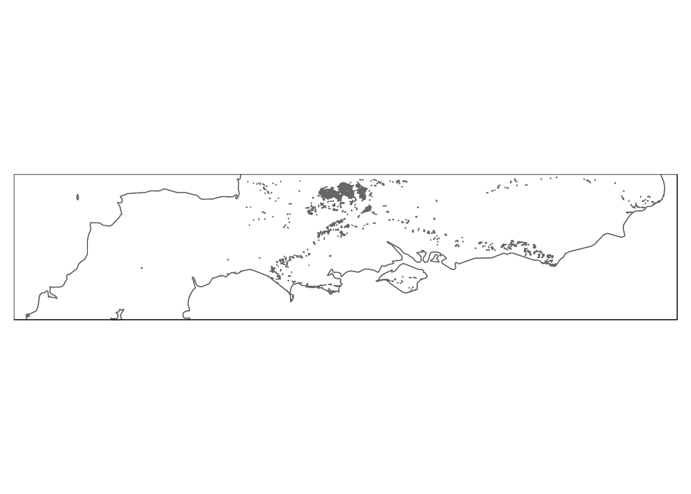
Figure 6.7: Calcareous grassland in the South of England.
6.3.9 Easy testing app
I have made a shiny app that you can use to test your understanding of spatial queries. The default table query fetches only the geometry in “safe mode” (i.e limited to a small number). You can then add attributes and type in conditions to filter on.
6.3.10 Conclusion
There is a lot more to SQL than these simple queries. The language can be very complex. However these examples are easy to follow and can form a template for extracting data from large data tables.