Chapter 16 Repeat measures designs
Repeated measures on the same experimental subject can occur for many reasons. The typical situation is when the measures are repeated in time, but repeated measures can also arise in other ways. The key to understanding when a design involves repeated measures is to realise that measures which involve different levels of the fixed factor of interest are taken from the same experimental unit. A blocked design is therefore an example of repeated measures in space if a block is regarded as an experimental unit. However blocks are usually thought of in terms of groups of experimental units. The terminology in the literature can be slightly confusing in this respect as it may depend on the discipline involved and blocked designs can be called repeated measures in some circumstances.
Let’s think of a simple example of a repeated measurement in a laboratory setting. The blood pressure of ten rats was measured before and after the injection of a drug.
library(lmerTest)
library(ggplot2)
library(effects)
library(reshape)
library(multcomp)
library(dplyr)d<-read.csv("https://tinyurl.com/aqm-data/rats.csv")Repeat measures such as these lead to a situation that is fundamentally similar to a design with blocks. Each treatment level is replicated once within each subject. However the total variability also has a between subject component as each rat may have a different baseline blood pressure. This needs to be taken into account.
g0<-ggplot(d,aes(x=time,y=resp))
g0+geom_boxplot()
g1<- g0+stat_summary(fun.data=mean_cl_normal,geom="point")
g1+stat_summary(fun.data=mean_cl_normal,geom="errorbar",colour="black")
16.1 Paired t-test
Just as in the blocked design failure to take into account between subject variability reduces the power of the analysis. We can see this by running two t-tests. The first is unpaired. The second is paired.
d2<-melt(d,id=1:2,m="resp")
d2<-cast(d2,id~time)
t.test(d2$Base,d2$Treat)
##
## Welch Two Sample t-test
##
## data: d2$Base and d2$Treat
## t = -1.2157, df = 16.68, p-value = 0.241
## alternative hypothesis: true difference in means is not equal to 0
## 95 percent confidence interval:
## -21.820632 5.881527
## sample estimates:
## mean of x mean of y
## 80.32928 88.29883t.test(d2$Base,d2$Treat,paired=TRUE)##
## Paired t-test
##
## data: d2$Base and d2$Treat
## t = -4.3212, df = 9, p-value = 0.00193
## alternative hypothesis: true difference in means is not equal to 0
## 95 percent confidence interval:
## -12.141652 -3.797453
## sample estimates:
## mean of the differences
## -7.96955216.2 Mixed effects model
The design can be analysed using a mixed effect model with rat id as a random effect.
First let’s see what happens if we don’t include the random effect.
mod<-lm(resp~time,data=d)
anova(mod)
## Analysis of Variance Table
##
## Response: resp
## Df Sum Sq Mean Sq F value Pr(>F)
## time 1 317.6 317.57 1.478 0.2398
## Residuals 18 3867.7 214.87You should see that the p-value is the same as we got from the unpaired t-test.
Now making rat id a random effect.
mod<-lmer(resp~time+(1|id),data=d)
summary(mod)
## Linear mixed model fit by REML. t-tests use Satterthwaite's method [
## lmerModLmerTest]
## Formula: resp ~ time + (1 | id)
## Data: d
##
## REML criterion at convergence: 135.4
##
## Scaled residuals:
## Min 1Q Median 3Q Max
## -1.42938 -0.49183 0.06957 0.55204 1.08978
##
## Random effects:
## Groups Name Variance Std.Dev.
## id (Intercept) 197.86 14.066
## Residual 17.01 4.124
## Number of obs: 20, groups: id, 10
##
## Fixed effects:
## Estimate Std. Error df t value Pr(>|t|)
## (Intercept) 80.329 4.635 9.740 17.329 1.21e-08 ***
## timeTreat 7.970 1.844 9.000 4.321 0.00193 **
## ---
## Signif. codes: 0 '***' 0.001 '**' 0.01 '*' 0.05 '.' 0.1 ' ' 1
##
## Correlation of Fixed Effects:
## (Intr)
## timeTreat -0.199par(mar=c(4,8,4,2))
plot(glht(mod))
Now the p-value is the same as that obtained by a paired t-test. Alternatively code this achieve the same result.
mod<-aov(resp~time+Error(id),data=d)
summary(mod)
##
## Error: id
## Df Sum Sq Mean Sq F value Pr(>F)
## Residuals 9 3715 412.7
##
## Error: Within
## Df Sum Sq Mean Sq F value Pr(>F)
## time 1 317.6 317.6 18.67 0.00193 **
## Residuals 9 153.1 17.0
## ---
## Signif. codes: 0 '***' 0.001 '**' 0.01 '*' 0.05 '.' 0.1 ' ' 1You should also be able to see the fundamental similarity between this situation and one involving blocking with respect to the specification of the model. However in a classic block design the blocks are considered to be groups of experimental units rather than individual experimental units. This can lead to confusion and model mispecification if you are not careful. A block design must have repeated measures with different levels of treatment within each block, just as a repeat measure design has different treatment levels within each subject. These simple examples can be extended to produce more complex designs.
16.3 Repeat measures with subsampling
One way the repeat measures design can be extended is with sub sampling. Take this example. A researcher is interested in the impact of sewage treatment plants outfalls on the diversity of river invertebrates. In order to produce a paired design kick samples are taken 100m above the outfall and 100m below the outfall in five rivers. This leads to a total of ten sites. At each site three kicks are obtained. These three measurements are thus sub-samples.
d<-read.csv("https://tinyurl.com/aqm-data/river.csv")
g0<-ggplot(d,aes(x=sewage,y=nspecies))
16.3.1 Visualising the data
If we pool all the data points taken below and above the sewage outfall we would not be taking into account the variability between rivers. We would also not be taking into account the potential for “pseudo-replication” as a result of the sub-sampling.
g0+geom_boxplot()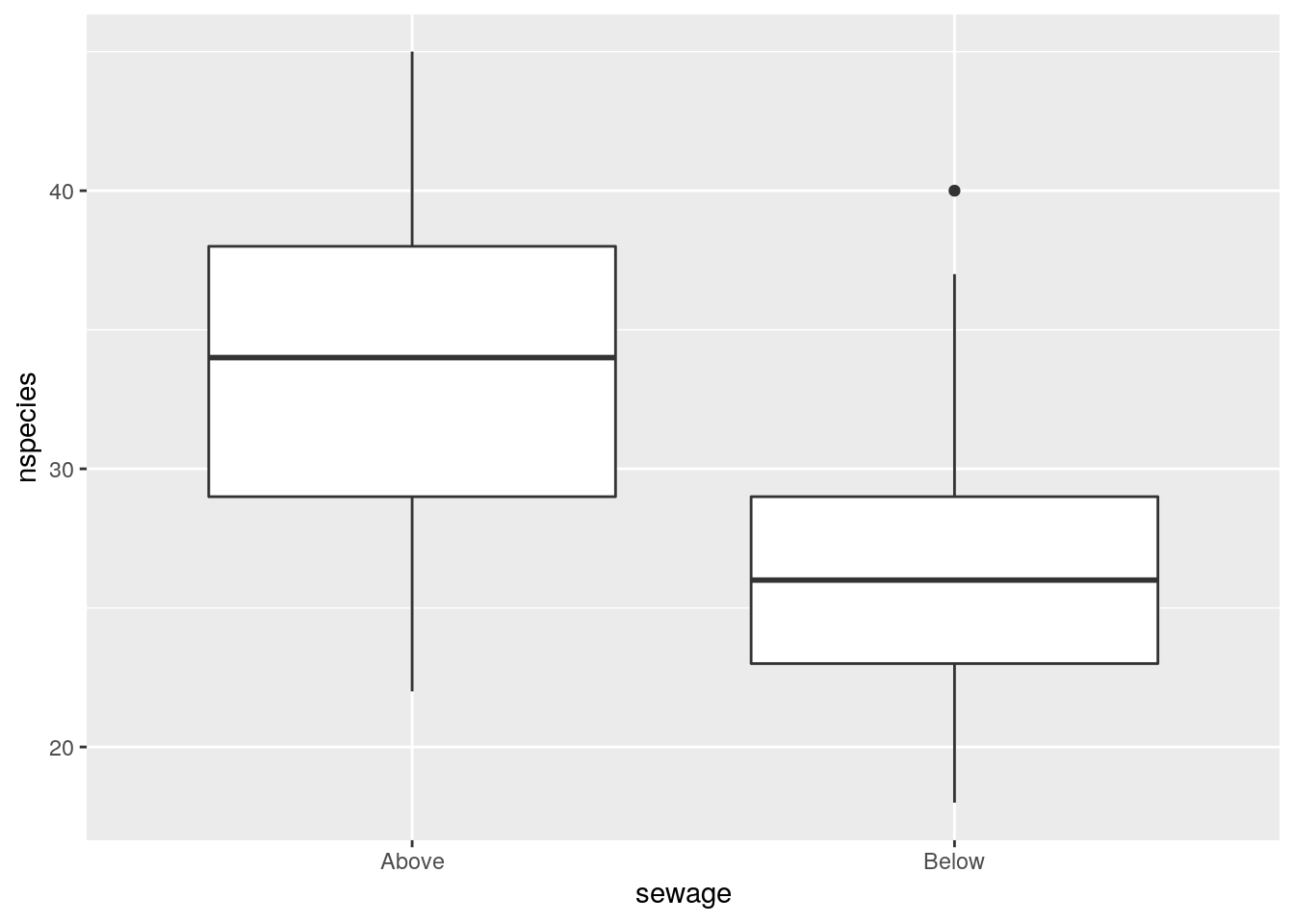
We can still obtain confidence intervals, but they would be based on a simplistic model that does not take into account the true data structure.
g1<-g0+stat_summary(fun.data=mean_cl_normal,geom="point")+stat_summary(fun.data=mean_cl_normal,geom="errorbar",colour="black")
g1
We could try splitting the data by river in order to visualise the pattern of differences.
g1+facet_wrap(~id)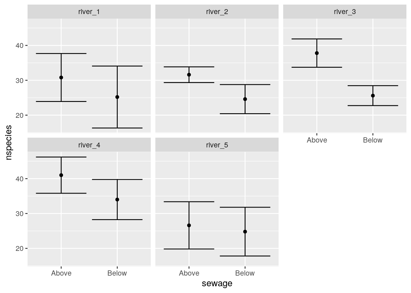
16.3.2 Incorrect model specification.
We could think of river id as a fixed effect. This may be reasonable if we are interested in differences between rivers. However it does not take into account the fact that the data consists of sub samples at each site. So the model below would be wrong.
mod<-lm(nspecies~sewage+id,data=d)
anova(mod)
## Analysis of Variance Table
##
## Response: nspecies
## Df Sum Sq Mean Sq F value Pr(>F)
## sewage 1 564.48 564.48 25.0596 9.454e-06 ***
## id 4 850.40 212.60 9.4382 1.344e-05 ***
## Residuals 44 991.12 22.53
## ---
## Signif. codes: 0 '***' 0.001 '**' 0.01 '*' 0.05 '.' 0.1 ' ' 116.3.3 Mixed effect model
The data could be modelled as nested random effects. There is random variability between rivers and there is also random variability between sites at each river. The fixed effect that we are most interested in concerns whether the site is above or below the sewage outfall.
mod<-lmer(nspecies~sewage+(1|id/site),data=d)
summary(mod)
## Linear mixed model fit by REML. t-tests use Satterthwaite's method [
## lmerModLmerTest]
## Formula: nspecies ~ sewage + (1 | id/site)
## Data: d
##
## REML criterion at convergence: 300.6
##
## Scaled residuals:
## Min 1Q Median 3Q Max
## -1.59547 -0.71758 -0.05326 0.60059 2.36669
##
## Random effects:
## Groups Name Variance Std.Dev.
## site:id (Intercept) 2.694 1.641
## id (Intercept) 17.789 4.218
## Residual 21.300 4.615
## Number of obs: 50, groups: site:id, 10; id, 5
##
## Fixed effects:
## Estimate Std. Error df t value Pr(>|t|)
## (Intercept) 33.560 2.225 5.272 15.086 1.54e-05 ***
## sewageBelow -6.720 1.668 4.001 -4.029 0.0157 *
## ---
## Signif. codes: 0 '***' 0.001 '**' 0.01 '*' 0.05 '.' 0.1 ' ' 1
##
## Correlation of Fixed Effects:
## (Intr)
## sewageBelow -0.375par(mar=c(4,8,4,2))
plot(glht(mod))
We could also treat river as a fixed effect if we are specifically interested in differences between rivers.
mod<-lmer(nspecies~sewage+id+(1|site),data=d)
anova(mod)
## Type III Analysis of Variance Table with Satterthwaite's method
## Sum Sq Mean Sq NumDF DenDF F value Pr(>F)
## sewage 345.7 345.7 1 4 16.2300 0.01575 *
## id 520.8 130.2 4 4 6.1127 0.05374 .
## ---
## Signif. codes: 0 '***' 0.001 '**' 0.01 '*' 0.05 '.' 0.1 ' ' 1summary(mod)## Linear mixed model fit by REML. t-tests use Satterthwaite's method [
## lmerModLmerTest]
## Formula: nspecies ~ sewage + id + (1 | site)
## Data: d
##
## REML criterion at convergence: 275.4
##
## Scaled residuals:
## Min 1Q Median 3Q Max
## -1.54770 -0.70432 -0.04561 0.61090 2.41441
##
## Random effects:
## Groups Name Variance Std.Dev.
## site (Intercept) 2.696 1.642
## Residual 21.300 4.615
## Number of obs: 50, groups: site, 10
##
## Fixed effects:
## Estimate Std. Error df t value Pr(>|t|)
## (Intercept) 31.360 2.043 4.000 15.350 0.000105 ***
## sewageBelow -6.720 1.668 4.000 -4.029 0.015751 *
## idriver_2 0.100 2.637 4.000 0.038 0.971572
## idriver_3 3.700 2.637 4.000 1.403 0.233304
## idriver_4 9.500 2.637 4.000 3.602 0.022718 *
## idriver_5 -2.300 2.637 4.000 -0.872 0.432392
## ---
## Signif. codes: 0 '***' 0.001 '**' 0.01 '*' 0.05 '.' 0.1 ' ' 1
##
## Correlation of Fixed Effects:
## (Intr) swgBlw idrv_2 idrv_3 idrv_4
## sewageBelow -0.408
## idriver_2 -0.645 0.000
## idriver_3 -0.645 0.000 0.500
## idriver_4 -0.645 0.000 0.500 0.500
## idriver_5 -0.645 0.000 0.500 0.500 0.500par(mar=c(4,8,4,2))
plot(glht(mod))
Notice that both models provide the same p-value for the effect of the sewage outfalls.
Using nested random effects produces an almost identical result to that which would be obtained by taking the means of the sub samples, as we have seen in previous examples.
# dd<-melt(d,m="nspecies") reshape method of aggregation
# dd1<-cast(dd,id+sewage~variable,mean)
## Dplyr method
d %>% group_by(id,sewage) %>% summarise(nspecies=mean(nspecies)) ->dd
## `summarise()` has grouped output by 'id'. You can override using the `.groups` argument.mod<-lm(nspecies~id+sewage,data=dd)
anova(mod)## Analysis of Variance Table
##
## Response: nspecies
## Df Sum Sq Mean Sq F value Pr(>F)
## id 4 170.080 42.520 6.1127 0.05374 .
## sewage 1 112.896 112.896 16.2300 0.01575 *
## Residuals 4 27.824 6.956
## ---
## Signif. codes: 0 '***' 0.001 '**' 0.01 '*' 0.05 '.' 0.1 ' ' 1