Chapter 3 Reading data into R from a web site
3.1 Introduction
Even research projects which aim to collect original field data frequently need to incorpoporate analyses of subsidiary data sets. It is common practice to download files and manipulate the data in Excel. This is acceptable. If you are familiar with Excel it can be convenient. However there are several drawbacks to using Excel
- The data manipulation is not clearly documented. If data have to be “cleaned” in Excel it is easy to lose track of the steps taken to achieve this. Using Excel can lead to multiple files and confusion regarding which is suitable for direct analysis.
- If the process needs to be repeated many times it can get very tedious and time consuming.
So, learning to useR to prepare data for analysis rather than Excel can eventually save a lot
library(DT)
library(tidyverse)
library(lubridate)
library(aqm)
3.2 Example. Reading data from the met office historical data site
Historical climate data for the UK is currently provided by the met office on this site.
https://www.metoffice.gov.uk/public/weather/climate-historic/#?tab=climateHistoric
If data is provided online in the form of a text table it is quite often possible to read it straight into R without downloading any files. Here is an example. We will load the data for the nearest station with a complete record directly.
3.3 Reading the raw file
If we read the file as lines we can see the structure, but we can not yet work directly with the data as lines.
d<-read_lines("https://www.metoffice.gov.uk/pub/data/weather/uk/climate/stationdata/hurndata.txt")
head(d,10)
## [1] "Hurn"
## [2] "Location 411700E 97800N, Lat 50.779 Lon -1.835, 10 metres amsl"
## [3] "Estimated data is marked with a * after the value."
## [4] "Missing data (more than 2 days missing in month) is marked by ---."
## [5] "Sunshine data taken from an automatic Kipp & Zonen sensor marked with a #, otherwise sunshine data taken from a Campbell Stokes recorder."
## [6] " yyyy mm tmax tmin af rain sun"
## [7] " degC degC days mm hours"
## [8] " 1957 1 9.1 2.5 7 73.0 ---"
## [9] " 1957 2 9.6 2.7 8 100.5 ---"
## [10] " 1957 3 12.9 5.5 4 61.3 ---"3.4 Reading the data to a data frame
The header of the file has some useful information. The first 5 lines are text. Then there is information for the column headers. However the info is split over two lines and line 7 has some gaps. The file is separated by tabs, not commas. We can see that because the text lines up with uniform gaps. So we choose the R command read_table to load the data, skipping the first 7 lines. Notice that the header also states that some additional symbols are used to mark missing data and estimated values. This quite often happens, but it can lead to unexpected and frustrating results. If a column being read into R contains any non numerical value at all then R will convert the values into a factor. We can check this by using “str”
d<-read.table("https://www.metoffice.gov.uk/pub/data/weather/uk/climate/stationdata/hurndata.txt",skip=7)
str(d)
## 'data.frame': 771 obs. of 7 variables:
## $ V1: int 1957 1957 1957 1957 1957 1957 1957 1957 1957 1957 ...
## $ V2: int 1 2 3 4 5 6 7 8 9 10 ...
## $ V3: Factor w/ 197 levels "0.4","10.0","10.1",..: 188 193 31 44 62 125 119 109 79 60 ...
## $ V4: Factor w/ 158 levels "-0.1","-0.2",..: 84 86 115 104 115 147 70 58 155 125 ...
## $ V5: Factor w/ 27 levels "0","1","10","10*",..: 25 26 22 14 2 1 1 1 2 14 ...
## $ V6: Factor w/ 568 levels "0.2","0.4","0.5",..: 460 12 412 347 316 225 477 461 474 396 ...
## $ V7: Factor w/ 556 levels "---","101.0",..: 1 1 1 1 1 1 1 1 1 1 ...3.5 Adding names
As we skipped the column headers we need to add them back.
names(d)<- c("Year", "Month", "tmax", "tmin", "af","rain", "sun") ## Add the headers 3.6 Cleaning the columns
If you are used to using Excel or Word you will be familiar with search and replace functions. Replacing characters in R is slightly more difficult, but much more powerful. The function to find and replace in a vector is gsub. Gsub works just like find and replace but can also use regular expressions. These are rule based expressions that can be written for specific purposes such as replacing all non-numeric characters.
Here is a useful little function that uses a regular expression to strip out all non numeric characters. Notice that the function also coerces factors first to a characters then to numerical values.
### A function to strip out any non numerical characters apart from the - and .
clean<-function(x)as.numeric(gsub("[^0-9.-]","",as.character(x)))
Now we can clean up the columns that should only contain numbers.
d$tmin<-clean(d$tmin)
d$tmax<-clean(d$tmax)
d$af<-clean(d$af)
d$rain<-clean(d$rain)
d$sun<-clean(d$sun)
## Warning in clean(d$sun): NAs introduced by coercion#write.csv(d,"/home/aqm/data/hurn.csv") ## Save locally on the server in case the web site goes offline
str(d)## 'data.frame': 771 obs. of 7 variables:
## $ Year : int 1957 1957 1957 1957 1957 1957 1957 1957 1957 1957 ...
## $ Month: int 1 2 3 4 5 6 7 8 9 10 ...
## $ tmax : num 9.1 9.6 12.9 14.2 16.1 22.2 21.6 20.6 17.8 15.9 ...
## $ tmin : num 2.5 2.7 5.5 4.4 5.5 8.8 12.9 11.7 9.6 6.6 ...
## $ af : num 7 8 4 2 1 0 0 0 1 2 ...
## $ rain : num 73 100.5 61.3 5.5 43.7 ...
## $ sun : num NA NA NA NA NA NA NA NA NA NA ...3.7 Making a date column
If data has a temporal component it should be turned into date format for use in R. There are many advantages to this, as
d$Month<- as.factor(d$Month)             ## Change the numeric variable to a factor
d$date<-as.Date( paste(d$Year,d$Month , 15 , sep = "/" )  , format = "%Y/%m/%d" )
The lubridate package provides many useful tricks for handling dates. For example, we may want to use names to the months.
d$month<-lubridate:::month(d$date,label=TRUE)3.8 Looking at the raw data
The dt function is a wrapper to the datatable function in the package DT. It is very useful for providing the data you are analysing in a downloadable format for others to use. When a document is knitted in RStudio the data itself is embedded in the document. If you are struggling to find a way to manipulate the data in R you can download it into a spreadsheet, change the data there, and start an analysis afresh with the new data. This is inefficient, but when you are starting out in R it may save time if you are used to spreadheets.
dt(d)3.9 Plotting the data
ggplot(d,aes(x=date,y=tmin)) + geom_line() +geom_smooth(col="red")
library(xts)
library(dygraphs)
Maxt<-xts(x = d$tmax, order.by = d$date)
Mint<-xts(x = d$tmin, order.by = d$date)
tmps<-cbind(Max_temp=Maxt,Min_temp=Mint)
 dygraph(tmps,group = "Hurn") %>% dyRangeSelector() %>% dyRoller(rollPeriod = 1)
3.10 Long to wide conversion
The data provided by the met office is in the correct “long” dataframe format. This makes data handling in R much simpler. However spreadsheet users often analyse data in a wide format. It is fairly simple to convert between the two data structures in R using the tidyverse.The wide format for tmin looks like this
d %>% select( c("Year","month","tmin")) %>% pivot_wider(names_from = "month", values_from="tmin") %>% dt()3.11 Disadvantages of the wide format
If the raw data had been provided in this wide format we would have had to import multiple tables, one for each variable. If data is held in spreadheets in a wide format it may be necessary to “reverse engineer” the data on each sheet to put it back into the correct data frame format. This can make data preparation a more lengthy process than it needs to be. So always hold your own data in the correct, long format, even if from time to time you may want to convert it to a wide format to share with others who do not use R and are used to calculating means and sums using Excel.
3.12 Using dplyr to summarise
The dplyr logic for summarising data is incredibly powerful once you get used to it. Modern R data manipulation makes a lot of use of the %>% operator. This is known as a pipe operator. What it does is to feed the data through a series of steps. The commonest use of dplyr involves grouping the dataframe then summarising it to produce a new data frame.
To get yearly summaries we first group_by year then summarise the variables using functions.
d %>% group_by(Year) %>% summarise(tmin=round(mean(tmin),2),tmax=round(mean(tmax),2),rain=sum(rain)) -> yrly
dt(yrly)
3.13 Exercise
Plot out the yearly date using ggplot.
3.14 Additional exercise
I have pre-processed spatial data from NASA’s MODIS based fire sensing site to show all the detected fires in the South of England
data("modisfires")
library(tmap)
qtm(south) + qtm(fires)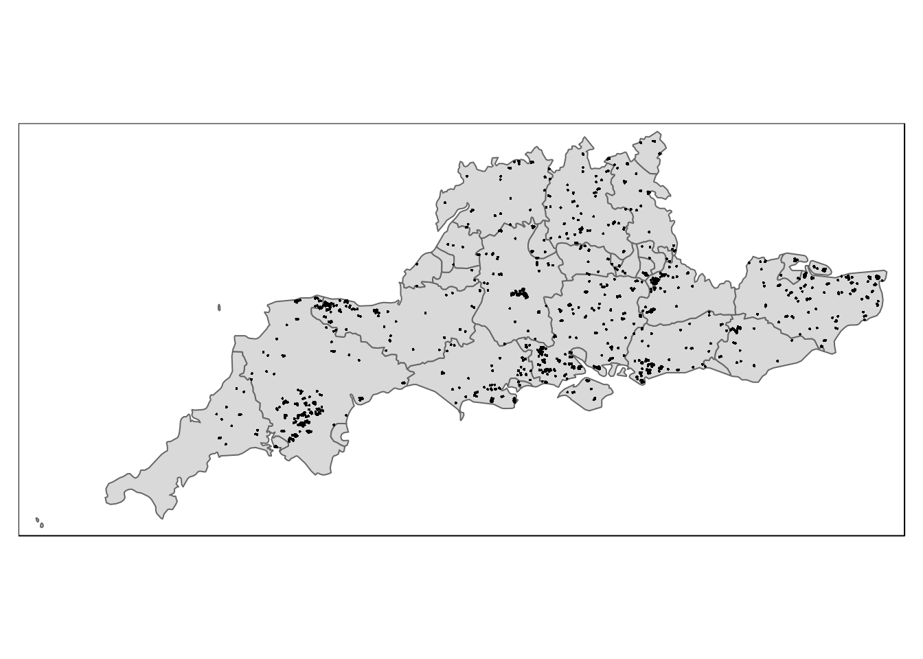
The number of fires can be joined to the yearly climate data.
yearly_fires%>% rename(Year=year) %>% inner_join(yrly) -> yearly_firesCan you find any relationship between the numbers of fires and the aggregated yearly climate data? If not, why might this not be the best way of looking for a relationship?
3.15 Repeating the operation
We can roll up all the data loading and cleaing steps above as a function which returns the data for the station as it is named on the web site. When the data on the site is updated to include recent months all that is required to update the data and all subsequent analysis based on it is to rerun the code.
I noticed that some stations have more lines that need to be skipped in the header (e.g Southampton).
f<-function(nm,skip=7)
{
URL<-sprintf("https://www.metoffice.gov.uk/pub/data/weather/uk/climate/stationdata/%sdata.txt",nm)
d<-read.table(URL,skip=skip, skipNul = TRUE, fill=TRUE,flush=TRUE)
names(d)<- c("Year", "Month", "tmax", "tmin",  "af","rain", "sun")
d$Year<-clean(d$Year)
d$tmin<-clean(d$tmin)
d$tmax<-clean(d$tmax)
d$af<-clean(d$af)
d$rain<-clean(d$rain)
d$sun<-clean(d$sun)
d$date<-as.Date( paste(d$Year,d$Month , 15 , sep = "/" )  , format = "%Y/%m/%d" )
d$month<-lubridate:::month(d$date,label=TRUE)
d$station<-nm
d
}
### I load each station by name as the raw data on the web site needs eyeballing first due to slight differences in format.
d1<-f("hurn")
d2<-f("yeovilton")
d3<-f("eastbourne")
d4<-f("southampton",skip=8)
d5<-f("camborne")
d6<-f("heathrow")
d7<-f("chivenor")
d8<-f("oxford")
d9<-f("eastbourne")
## Add a contrast
d10<-f("braemar",skip=8)
d<-rbind(d1,d2,d3,d4,d5,d6,d7,d8,d9,d10)
write.csv(d,"/home/aqm/data/met_office.csv")
str(d)
## 'data.frame': 9627 obs. of 10 variables:
## $ Year : num 1957 1957 1957 1957 1957 ...
## $ Month : chr "1" "2" "3" "4" ...
## $ tmax : num 9.1 9.6 12.9 14.2 16.1 22.2 21.6 20.6 17.8 15.9 ...
## $ tmin : num 2.5 2.7 5.5 4.4 5.5 8.8 12.9 11.7 9.6 6.6 ...
## $ af : num 7 8 4 2 1 0 0 0 1 2 ...
## $ rain : num 73 100.5 61.3 5.5 43.7 ...
## $ sun : num NA NA NA NA NA NA NA NA NA NA ...
## $ date : Date, format: "1957-01-15" "1957-02-15" ...
## $ month : Ord.factor w/ 12 levels "Jan"<"Feb"<"Mar"<..: 1 2 3 4 5 6 7 8 9 10 ...
## $ station: chr "hurn" "hurn" "hurn" "hurn" ...met_office<-d
dt(d)#save(d,met_office,file="~/rstudio/aqm/data/met_office_2021.rda")3.16 Get lattitude and Longitude
This is a bit tricky but can be done. Don’t try to follow any of this, just use the results.
library(stringr)
f2<-function(nm="hurn",line=2) {
URL<-sprintf("https://www.metoffice.gov.uk/pub/data/weather/uk/climate/stationdata/%sdata.txt",nm)
d<-read_lines(URL)
Lat<-clean(str_match(d[line], "Lat\\s*[+-]?([0-9]*[.])?[0-9]+")[,1])
Lon<-clean(str_match(d[line], "Lon\\s*[+-]?([0-9]*[.])?[0-9]+")[,1])
data.frame(station=nm,Lat=Lat,Lon=Lon)
}
d1<-f2("hurn")
d1<-rbind(d1,f2("yeovilton"))
d1<-rbind(d1,f2("eastbourne"))
d1<-rbind(d1,f2("southampton",line=3))
d1<-rbind(d1,f2("camborne"))
d1<-rbind(d1,f2("heathrow"))
d1<-rbind(d1,f2("chivenor"))
d1<-rbind(d1,f2("oxford"))
d1<-rbind(d1,f2("eastbourne"))
d1<-rbind(d1,f2("braemar",line=3))
d1
## station Lat Lon
## 1 hurn 50.779 -1.835
## 2 yeovilton 51.006 -2.641
## 3 eastbourne 50.762 0.285
## 4 southampton 50.898 -1.408
## 5 camborne 50.218 -5.327
## 6 heathrow 51.479 -0.449
## 7 chivenor 51.089 -4.147
## 8 oxford 51.761 -1.262
## 9 eastbourne 50.762 0.285
## 10 braemar 57.006 -3.396#write.csv(d1,"~/rstudio/aqm/inst/extdata/met_office_coords.csv")library(mapview)
library(sf)
d1<-st_as_sf(d1, coords = c("Lon", "Lat"), crs = 4326)
mapview(d1, legend=FALSE)