Chapter 12 Non-linear models
Statistical modelling involves measures of fit. However scientific modelling often brings in other elements, including theory that is used to propose a model for the data. These theoretical models are often non-linear in the statistical sense. The terms do not enter in a linear manner. Such models can be difficult to fit to real life data, but are often used when building process based ecological models.
12.1 Fitting a rectangular hyperbola
For example, resource use is commonly modelled using a function with an asymptote. The equation below is a version of Holling’s disk equation that has been rewriten as a generalised rectangular hyperbola. This is identical in form to the Michaelis-Menton equation for enzyme kinetics.
\[C=\frac{sR}{F+R}\]
Where
- C is resource consumption,
- R is the amount or density of theresource,
- s is the asymptotic value and
- F represents the density of resource at which half the asymptotic consumption is expected to occur. This model is not linear in its parameters.
The data below have been simulated from this equation in order to illustrate the model fitting process.
d<-read.csv("/home/aqm/course/data/Hollings.csv")
plot(d,pch=21,bg=2)
There are many ways to fit a theoretical non-linear model in R. One of the simplest uses least squares, so some of the assumptions made are similar to linear regression.
It is much harder to run diagnosis on these sorts of models. Even fitting them can be tricky. Diagnostics are arguably less important, as the interest lies in finding a model that matches our understanding of how the process works, rather than fitting the data as well as possible.
We have to provide R with a list of reasonable starting values for the model. At present R does not provide confidence bands for plotting, but this is less important in the case of non linear models. It is much more interesting to look at the confidence intervals for the parameters themselves.
nlmod<-nls(Consumption~s*Resource/(F+Resource),data = d,start = list( F = 20,s=20))
newdata <- data.frame(Resource=seq(min(d$Resource),max(d$Resource),l=100))
a <- predict(nlmod, newdata = newdata)
plot(d,main="Non-linear model")
lines(newdata$Resource,a,lwd=2)
confint(nlmod)## Waiting for profiling to be done...## 2.5% 97.5%
## F 33.97300 43.66697
## s 19.58576 20.32930g0<-ggplot(data=d,aes(x=Resource,y=Consumption))
g1<-g0+geom_point()
g1+geom_smooth(method="nls",formula=y~s*x/(F+x),method.args=list(start = c( F = 20,s=20)), se=FALSE)
The nice result of fitting this form of model is that we can now interpret the result in the context of the process. If the resource represented biomass of ragworm in mg m2 and consumption feeding rate of waders we could now estimate the maximum rate of feeding lies between 19.5 and 20.3 mg hr. The density at which birds feed at half this maximum rate, if the theoretical model applies, lies beyond the range of the data that we obtained (34 to 44 mg m2).
Non linear models can thus be extrapolated beyond the data range in a way that linear models, polynomials and splines cannot. However this extrapolation relies on assuming that the functional form of the model is sound.
It is common to find that parameters are estimated with very wide confidence intervals even when a model provides a good fit to the data. Reporting confidence intervals for key parameters such as the asymptote is much more important in this context than reporting R2 values. This can be especially important if the results from non linear model fitting are to be used to build process models.
You should not usually fit a non-linear model of this type to data, unless you have an underlying theory. When the data are taken from a real life situation it is always best to explore them first using other approaches before thinking about fitting a non-linear model. When we obtain data from nature we do not know that the equation really does represent the process. Even if it does, there will certainly be quite a lot of random noise around the underlying line.
12.2 Real data
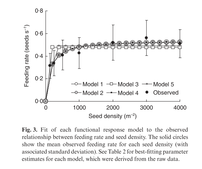
Smart, Stillman and Norris were interested in the functional responses of farmland birds. In particular they wished to understand the feeding behaviour of the corn bunting Miliaria calandra L, a bird species whose decline may be linked to a reduction of food supply in stubble fields.
The authors tested five alternative models of the functional responses of corn buntings. They concluded that Holling’s disk equation provided the most accurate fit to the observed feeding rates while remaining the most statistically simple model tested.
d<-read.csv("/home/aqm/course/data/buntings.csv")

plot(rate~density,data=d,pch=21,bg=2)
The classic version of Hollings disk equation used in the article is written as
\[ R=\frac{aD}{1+aDH} \]
Where
- F = feeding rate (food items)
- D = food density (food items \(m^{-2}\))
- a = searching rate (\(m^{2}s^{-1}\))
- H = handling time (s per food item).
HDmod<-nls(rate~a*density/(1+a*density*H),data = d,start = list(a =0.001,H=2))
confint(HDmod)
## Waiting for profiling to be done...## 2.5% 97.5%
## a 0.002593086 0.006694939
## H 1.713495694 1.976978655newdata <- data.frame(density=seq(0,max(d$density),l=100))
HDpreds <- predict(HDmod, newdata = newdata)
plot(rate~density,data=d,pch=21,bg=2,ylim=c(0,1))
lines(newdata$density,HDpreds,lwd=2)
g0<-ggplot(data=d,aes(x=density,y=rate))
g1<-g0+geom_point()
g1+geom_smooth(method="nls",formula=y~a*x/(1+a*x*H),method.args=list(start = c(a = 0.01,H=2)), se=FALSE)
The figure in the article shows the five models that were considered.
alt
Note that models with a vigilance term could not be fit to the data directly due to lack of convergence.
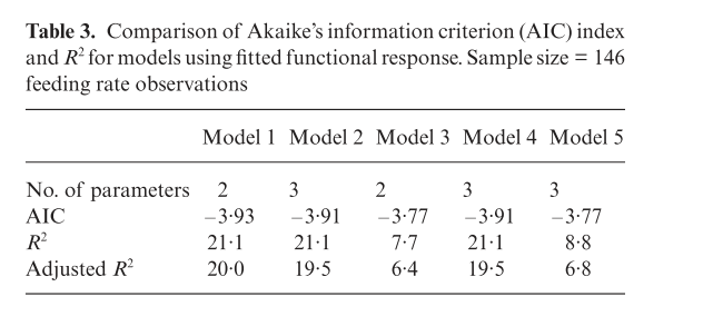
12.2.1 Calculating the R squared
The fit of the models in the paper is presented below.
alt
R does not calculate R squared for non linear models by default. The reason is that statisticians do not accept this as a valid measure. However ecologists are used to seeing R squared values when models are fit. You can calculate them easily enough from a non linear model. First you need the sum of squares that is not explained by the fitted model. This is simply the variance multiplied by n-1.
nullss<-(length(d$rate)-1)*var(d$rate)
nullss
## [1] 3.544056We get the residual sum of squares (i.e. the unexplained variability) when we print the model
HDmod## Nonlinear regression model
## model: rate ~ a * density/(1 + a * density * H)
## data: d
## a H
## 0.003966 1.841890
## residual sum-of-squares: 2.795
##
## Number of iterations to convergence: 7
## Achieved convergence tolerance: 3.807e-06So, R squared is just one minus the ratio of the two.
Rsq<-1-2.795/nullss
Rsq*100
## [1] 21.13555Which agrees with the value given in the paper.
12.2.2 Including the vigilance term
A very interesting aspect of this article is that the terms of the model were in fact measured independently.
Vigilance, which is defined as the proportion of the time spent being vigilant, rather than feeding, is included in most of the models which are presented in the paper as alternatives to the classic disk equation. Most of these are rather complex conditional models, but the simplest is model 2.
\[ R=\frac{(1-v)aD}{1+aDH} \]
The vigilance parameter for model2 cannot be estimated from the data. However it was also measured independently.
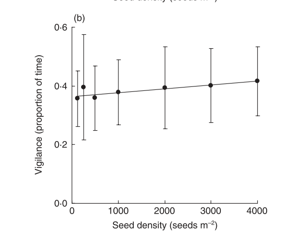
alt
Notice that vigilance is fundamentally independent of seed density within this range of densities. The measured value (approximately 0.4) can be included and the model refit with this value included.
Vigmod<-nls(rate~(1-0.4)*a*density/(1+a*density*H),data = d,start = list(a =0.001,H=2))
confint(Vigmod)
## Waiting for profiling to be done...## 2.5% 97.5%
## a 0.004321811 0.01115823
## H 1.028097415 1.18618719When the measured vigilance is included in the model as an offset term the handling time is reduced by about a half. This makes sense. We may assume that most of the measured vigilance is in fact reducing the rate of feeding as the seed density is so high that search time is very small. However note that we could not possibly have fitted this model without some prior knowledge of the offset value.
12.3 Quantile regression
Another way to look at the issue is to use an alternative approach to fitting statistical models. The traditional approach to fitting a model to data assumes that we are always interested in the centre of any pattern. The error term was classically assumed to be uninteresting random noise around an underlying signal. However in many situations this noise is actually part of the phenomenon we are studying. It may sometimes be attributed to process error, in other words variability in the process we are actually measuring, rather than error in our measurements. This may possibly be occurring here. If handling time in fact sets an upper limit on feeding rate, and if we can assume that feeding rate has been measured fairly accurately, then the upper part of the data cloud should be estimating true handling time. Birds that are feeding more slowly than this may be doing something else. For example, they may be spending time being vigilant. So there is possibly some additional information in the data that has not been used in the published paper.
We can use quantile regression to fit a non linear model around the top 10% of the data and the bottom 10%.
library(quantreg)## Loading required package: SparseM##
## Attaching package: 'SparseM'## The following object is masked from 'package:base':
##
## backsolveQuantMod90<-nlrq(rate~a*density/(1+a*density*H),data = d,start = list(a =0.001,H=2),tau=0.9)
QuantMod10<-nlrq(rate~a*density/(1+a*density*H),data = d,start = list(a =0.001,H=2),tau=0.1)
QuantPreds90 <- predict(QuantMod90, newdata = newdata)
QuantPreds10 <- predict(QuantMod10, newdata = newdata)
plot(rate~density,data=d,pch=21,bg=2,ylim=c(0,1))
lines(newdata$density,HDpreds,lwd=2, col=1)
lines(newdata$density,QuantPreds90,lwd=2,col=2)
lines(newdata$density,QuantPreds10,lwd=2,col=3)
If handling time limits the maximum rate at which seed can be consumed, then the estimate based on the upper 10% of the data should be closer to the true handling time. So if we look at the summaries of these models we should be able to get a handle on vigilance without the prior knowledge.
summary(QuantMod90)##
## Call: nlrq(formula = rate ~ a * density/(1 + a * density * H), data = d,
## start = list(a = 0.001, H = 2), tau = 0.9, control = list(
## maxiter = 100, k = 2, InitialStepSize = 1, big = 1e+20,
## eps = 1e-07, beta = 0.97), trace = FALSE)
##
## tau: [1] 0.9
##
## Coefficients:
## Value Std. Error t value Pr(>|t|)
## a 0.00821 0.00111 7.37199 0.00000
## H 1.37329 0.04741 28.96694 0.00000summary(QuantMod10)##
## Call: nlrq(formula = rate ~ a * density/(1 + a * density * H), data = d,
## start = list(a = 0.001, H = 2), tau = 0.1, control = list(
## maxiter = 100, k = 2, InitialStepSize = 1, big = 1e+20,
## eps = 1e-07, beta = 0.97), trace = FALSE)
##
## tau: [1] 0.1
##
## Coefficients:
## Value Std. Error t value Pr(>|t|)
## a 0.00117 0.00052 2.25050 0.02593
## H 2.64950 0.29590 8.95388 0.00000The upper limit (pure handling time) is 1.37 (se= 0.047)
The lower estimate that may include time spent being vigilant is estimated using quantile regression as 2.65 (se= 0.31)
Vigilance thus could, arguably, be estimated as the difference between the upper and lower estimates of handling time divided by the upper value. As the uncertainty around these values has been provided by the quantile regression in the form of a standard error we can use a montecarlo prodedure to find confidence intervals by simulating from the distributions and finding the percentiles of the result.
quantile((rnorm(10000,2.65,0.31)-rnorm(10000,1.37,0.047))/rnorm(10000,2.65,0.31),c(0.025,0.5,0.975))## 2.5% 50% 97.5%
## 0.2487116 0.4829750 0.7766975This is within the range of the measured value.
There are some interesting elements here that could be discussed in the context of the explanation of the study methods and results.
12.4 Summary
Many relationships in ecology do not form strait lines. If we only have data, and no underlying theory, we can fit a model to the underlying shape using traditional methods such as polynomials or more contemporary models such as splines and other forms of local weighted regression. However these models cannot be extrapolated beyond the data range.
A very different approach involves finding a model “from first principles”. Often models are constrained to pass through the origin and by some fundamental limit (asymptote). Model fitting then involves finding a justifiable form for the curve lying between these two points. In some situations data can be used to “mediate” between competing models. In other situations the best we can achieve is to find justifiable estimates, with confidence intervals, for the parameters of a non linear model.
12.5 Exercise
A researcher is interested in establishing a predicitive equation to estimate the heights of trees based on measurements of their diameter at breast height. Your task is to try to find a defensible model for three different data sets.
pines1<-read.csv("https://tinyurl.com/aqm-data/pinus_allometry1.csv")oaks<-read.csv("https://tinyurl.com/aqm-data/quercus_allometry.csv")pines2<-read.csv("https://tinyurl.com/aqm-data/pinus_allometry2.csv")